Animal Location Tracker (A3032)
© 2016-2020 Kevan Hashemi,
Open Source Instruments Inc.
Contents
Description
Design
Set-Up
Current Consumption
Modifications
Feasibility Study
Development
Description
[03-OCT-19] The Animal Location Tracker (ALT, assembly A3032) is a LWDAQ device that provides a horizontal array of fifteen detector coils to measure the position of subcutaneous transmitters (SCT). The ALT is designed to measure the activity of animals in cages, and to disambiguate video of animals in cages. The activity of an animal is the distance it moves. We might measure activity in each second, or in each minute. The disambiguation of video is the determination of which animal is which in the field of view of the camera, when all animals look similar. To track the movements of animals, the ALT uses the signals transmitted by Subcutaneous Transmitters (SCT) implanted in the animals on the platform. We measure the approximate location of a transmitter by looking at the power received by each of the detector coils. We measure activity by tracing the path made by consecutive ALT position measurements. We disambiguate video by correlating the movements measured by the ALT with those we obtain from blob-tracking analysis of video recorded by our Animal Cage Cameras (ACC). Each SCT has its own unique channel number, so each animal has its own unique location and velocity.
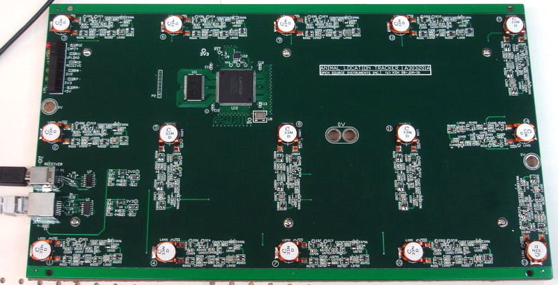
Figure: Animal Location Tracker (A3032A) Circuit Board. Fifteen detector coils and amplifiers are arranged on a 32 cm × 16 cm grid. The LWDAQ socket is on the lower left, just below a USB socket for connection to an Octal Data Receiver. There are six indicator lights on the top-left. From the top they are: Message Buffer Empty (red), Uploading Data (yellow), Receiving Notifications (green), +3.3 V Power (green), +3.0 V Power (green), and +5 V Power (green).
Our SCTs emit 7-μs bursts of electromagnetic radiation in the range 902-928 MHz. Each detector coil provides a measurement of magnetic field strength in this same frequency range. The A3032 does not decode SCT messages itself. It relies upon an Octal Data Receiver (A3027) to decode the messages. The A3027 must be equipped with a location-tracking version of the A3027 firmware. We connect the receiver to the tracker with a USB cable (USB-A to USB-B).
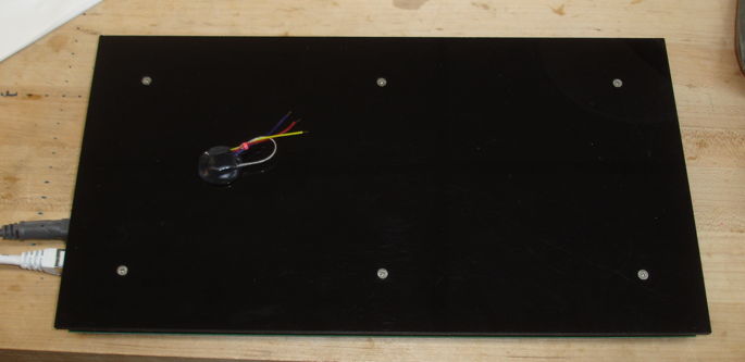
Figure: Animal Location Tracker (A3032A) Platform. We place an animal cage on top, with SCTs implanted in cage inhabitants. The platform is 34 cm × 18 cm.
When an SCT message is in progress, the receiver instructs the tracker to take power measurements from all coils. When an SCT message is complete and correct, the receiver transmits the SCT message channel number, contents, and time stamp to the tracker. The tracker saves these four bytes to its memory, followed by fifteen bytes of detector coil measurements and a firmware byte. We download the samples and the power measurements together with the Receiver Instrument in the LWDAQ Software. We store the tracker data to disk with the Neuroarchiver Tool. The Neuroarchiver contains a Tracker button that opens the Neurotracker Panel, which displays the position of SCTs on the tracker platform.
Figure: Neurotracker Panel Provided by the Neuroarchiver. Default parameters to control the location calculation are shown along the top.
The absolute accuracy of the ALT in measuring position of an SCT in a beaker of water or implanted in an animal with respect to the coordinate system defined by its coil centers is ±2 cm 90% of the time, and ±10 cm the rest of the time. Because there is no way to know whether the absolute position is accurate or not, the absolute measurement provided by the ALT is not useful on its own as a way to monitor animal position. The ALT's measurement of the direction and magnitude of movement, however, is far more useful. Its measurement of the change in an animal's position allows us to measure an animal's activity, and also to identify which animal is which in video. The correlation between ALT movement and video blob-tracking permits us to be 100% certain which blob corresponds to which animal, even when there are a dozen animals in the field of view.
| Version |
X (cm) |
Y (cm) |
Coil Pitch (cm) |
Coil Type |
Num Coils |
Comment |
| A3032A |
32 |
16 |
8 |
257 nH SMT |
15 |
100.0% accurate disambiguation for height 0-5 cm. |
| A3032B |
40 |
24 |
8 |
7-cm diameter loop |
15 |
99.0% accurate disambiguation for height 0-5 cm. |
| A3032C |
32 |
16 |
8 |
33 nH SMT |
15 |
100.0% accurate disambiguation for height 0-5 cm. |
Table: Versions of the A3032.
The only version in production now is the A3032C, the other versions having been converted to A3032Cs.
Design
S3032_1: Power Detectors 01-15.
S3032_2: LVDS Transceivers.
S3032_3: Logic and Memory.
A303201A: Gerber files for printed circuit board version A.
A303201A: Multi-layer view of printed circuit board version A.
A303201A_Top: Drawing of top side of printed circuit board version A.
A3032A.ods: BOM and Pick-and-Place for A3032A.
LT5534: Radio-frequency power detector.
LAT-3+: 3-dB attenuator.
ADC081S101: Eight-bit serial ADC.
UPC2746: Low-power 18-dB 900-MHz amplifier.
2014VS: Vertical, surface-mount inductor.
Set-Up
Note: These set-up instructions assume you are using LWDAQ 9.1.7+. Download and install the latest version here
[18-DEC-19] The figure below shows two Animal Location Tracker (A3032A) platforms included in a larger fourteen-animal SCT System.
Figure: Animal Location Trackers Operating with Subcutaneous Transmitter System. A data acquisition computer (1) is connected via a TCPIP network (2) to a LWDAQ Driver (3), which receives power from a 24-V adaptor (4). Three shielded CAT-5 cables (5) provide power and communication to the Octal Data Receiver (6) and the two Animal Location Trackers (10). Eight coaxial cables (7) carry antenna signals to the Octal Data Receiver amplifier inputs. Loop antennas (8) pick up signals from implanted transmitters. Three faraday enclosures (9) isolate a total of fourteen animals from other SCT systems and from local radio-frequency interference. Six animals are living on two ALT platforms (10). The ALTs are connected to the Octal Data Receiver with USB cables (11). All cables within the faraday enclosures are shielded cables and pass through grounded feedthrough connectors (12) at the wall of the enclosure.
To set up an ALT in an SCT system, take the following steps. If you need help setting up the SCT system itself, see SCT System Set-Up.
- Install Feed-Through Connectors: These go in the faraday enclosure walls. You will need new holes in the faraday enclosure to accommodate the feedthroughs. If you don't have the holes drilled yet, you can run the cables through a partly-open enclosure door straight to the ALT. When you embark upon a long-term recording, however, we recommend you be able to close the door completely. There are two feedthrough connectors for each ALT. One is USB-A to USB-B, the other is an RJ-45 to RJ-45. The USB feedthrough should have its USB-A plug on the inside of the faraday enclosure. Within the faraday enclosure, use a 1-m long USB-A to USB-B cable and a 1-m long shielded CAT-5 ethernet cable to connect the ALT to the feedthroughs.
- Connect ALT to LWDAQ Driver: Use a shielded CAT-5 ethernet cable to connect an empty driver socket on the LWDAQ Driver to the ALT's RJ-45 feedthrough. The driver sockets are the ones below the line of indicator lamps. There are eight driver sockets on the A2071E or A2037E LWDAQ Drivers. They are numbered 1-8, with 1 being closest to the lights.
- Connect ALT to Octal Data Receiver: Connect the Octal Data Receiver to the ALT's USB feedthrough with a USB cable. Plug the cable into either the Y1 or Y2 ports on the Octal Data Receiver. The ALT does not detect and decode SCT messages itself. Instead, it receives notifications of message activity from the Octal Data Receiver via a USB cable.
- Check Octal Data Receiver Firmware Version: If you are recording from your Octal Data Receiver with LWDAQ, open the Receiver Instrument and check the FV field. The firmware version should be ≥9. If there is no such LWDAQ instance, start LWDAQ, open the Receiver Instrument, set daq_ip_addr and daq_driver_socket to point to the Octal Data Receiver. Press Reset and then Acquire. Check that FV ≥9. If FV ≤ 8, we need to your receiver's firmware: return the receiver to us for an update, or follow our firmware reprogramming instructions.
- Check LWDAQ Driver Software Version: We can record simultaneously and independently from both ALTs and the data receiver. To do so reliably, you will need a LWDAQ Driver with software version ≥15. Open the Configurator Tool and enter the IP address of your LWDAQ Driver. Press Contact. Check the software version number the Configurator displays is ≥15.
- Contact ALT: Open the Receiver Instrument in an instance of LWDAQ dedicated to recording from one of the ALTs. Set daq_driver_socket and daq_ip_addr to point to the ALT. Set payload_length to 16 to suit the messages provided by the ALT. Press Reset. You should see the red Empty light flash once on the ALT. The green Receive light should be on, as well as all three power lights. If not, try pressing the hardware reset button on the front face of the LWDAQ Driver. But be aware that resetting the LWDAQ Driver will temporarily interrupt any other recordings.
- Download from ALT: In the Receiver Instrument, press Reset and then Loop. You should see the signal traces from every transmitter being recorded by the Octal Data Receiver, whether it is on the ALT or not.
- Record from ALT: Open the Neuroarchiver Tool. In the recorder section, set the IP and Socket fields to point to your ALT. Select "A3032" in the version menu button. Select a recording directory, press Reset, with for the reset to complete, and press Record. Transmitter messages with a payload of sixteen bytes of power measurements are now being downloaded from the ALT and written to an NDF file on disk. In the player section, select this same file and play it. You should see the signal traces from the subcutaneous transmitters displayed in the Neuroarchiver plots. In the select box, enter the channel numbers of the transmitters that are over the tracking platform, so you can isolate these from the others. Press Tracker and you should see the locations of all transmitters on the platform displayed.
Because the NDF file created by the Neuroarchiver from the ALT data contains the raw power measurements made by the ALT, you can go back later, re-play the data and re-calculate SCT movements.
Current Consumption
The A3032A consumes 280 mA from the LWDAQ +5-V power supply, and nothing from the LWDAQ ±15-V power supplies. The LWDAQ Driver (A2071E) can deliver 2000 mA at +5 V and 500 mA at ±15 V. An Octal Data Receiver (A3037E) consumes 510 mA from +5 V and 330 mA from ±15 V. Provided you use LWDAQ Software version 8.4.3+, you can connect two A3032A to one A3027E with two USB cables and record from all three devices simultaneously with the Neuroarchivers in three separate instances of the LWDAQ Software. Provided your LWDAQ Driver (A2071E) has software version 15 or higher, it provides a queu for socket connections and executes them in turn. If we assume fourteen 512 SPS SCTs being picked up by the A3027E, we have 20 bytes for each sample from each A3032A and four bytes from the A3027E makes around 300 KBytes/s. The maximum download rate from the driver is 1.4 MBytes/s.
Modifications
The footprint for P1 is incorrect in the A303201A printed circuit board. We must cut tracks and make the connections shown below.
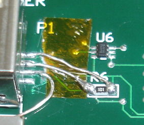
Figure: P1 Modification on A303201A.
No other modifications are required by the A3032A using the A303201A circuit board.
Feasibility Study
[01-MAR-16] We investigate the effect of orientation, antenna length, and material environment upon power received by a nearby Loop Antenna (A3015C). We start by wrapping the 150-mm leads of the transmitter around the transmitter body, then laying them out straight, then wrapping them around the antenna like this. The state of the leads has less than a ±2 dB effect upon the received power. We cut the leads back to 20 mm to simplify our subsequent measurements. We place an A3028E in a petri dish on top of a horizontal loop antenna and rotate the petri dish, measuring power received by the antenna using our Spectrometer (A3008). We measure power in dBm, which is decibels relative to 1 mW, so −30 dBm is 1 μW and −60 dBm is 1 nW. The threshold for reliable reception in a faraday enclosure is −60 dBm, and for outside a faraday enclosure in our office is −30 dBm.
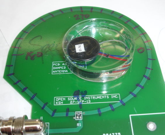
Figure: Apparatus for Measuring Received Power with Rotation at Zero Range, In Water and In Air. This is the zero rotation.
We rotate the A30128E in air with 50-mm loop antenna. We add water to the petri dish and repeat. We cut back the antenna to 40 mm, then 30 mm, making a loop out of the antenna in each case. We cut back to 20 mm and let the antenna stick out straight.
Figure: Received Power at Zero Range with Rotation in Plane Perpendicular to Receive Antenna, for Various Antenna Lengths, Loop and Straight, in Water and in Air. The plot shows received power in dBm versus rotation, with zero rotation at the top, and clockwise rotation in the plot being clockwise rotation of the antenna seen from above.
We place a vertical spectrometer antenna 20 cm from the rotating transmitter, with the loop facing the transmitter. The transmit antenna is in a horizontal plane, while the receive antenna is in a vertical plane. The distance between the two is similar to the distance between an implanted transmitter and a receive antenna outside its cage.
Figure: Received Power at 20-cm Range with Rotation in Plane Perpendicular to Receive Antenna, for Rat and Mouse (R/M) Transmitters in Air, Propanol, and Water (A/P/W). The rat antenna is 50 mm and the mouse antenna is 30 mm.
In our next test, we compare the 20-mm straight antenna's performance in air and water. We can orient the antenna axis vertically by placing the antenna in a small beaker, either full of water or empty. In this way, we compare the 50-mm loop antenna when vertical and horizontal.
Figure: Received Power at 20-cm Range with Rotation in Plane Perpendicular to Receive Antenna, for Rat Transmitters in Air and Water (A/W) with 50-mm Loop and 20-mm Straight Antennas (50/20), and Horizontal and Vertical Orientation (H/V).
If we have two independent receive antennas to pick up the signal of our transmitter, we will do better if we orient them so that their faces are perpendicular. With three mutually perpendicular antennas, there is no orientation of the transmit antenna axis that is parallel to all three planes.
[04-MAR-16] We compare the A3028E's 50-mm loop antenna with a 50-mm straight antenna. We start with a loop, then release the end of the loop to create a straight antenna.
Figure: Received Power at 20-cm Range with Rotation in Plane Perpendicular to Receive Antenna, for 50-mm Antennas Straight and Bent (S/B), Horizontal and Vertical Orientation (H/V), in Air and Water (A/W). When submerged in water, the antenna is just beneath the surface of a 10-mm deep pool.
When we rotate the straight antenna in the vertical orientation, we are rotating it about its own axis, so we expect no dramatic changes in received power. The body of the transmitter is rotating, and it plays a part in the transmission, so we see some variation in received power. In the horizontal orientation, the emission pattern of the straight antenna has two deep, sharp minima, both in water and in air. The bent antenna has one sharp minimum in air, and no sharp minimum in water.
We place the receive antenna below our work bench at range 20 cm from our rotating transmitter. We rotate bent and straight antennas in water and air.
Figure: Received Power at 20-cm Range with Transmit Antenna Rotating in Plane Parallel to Receive Antenna, for 30-mm and 50-mm Antennas (30/50), Straight and Bent (S/B), in Air and Water (A/W). When submerged in water, the antenna is just beneath the surface of a 10-mm deep pool.
We tie a transmitter to a latex glove full of water, so as to simulate implantation outside the skin of an animal, see here. Later, we put the transmitter inside the glove with the water, pressed up against the top side, as if implanted subcutaneously. The antenna loop is rotated about its axis so that the loop is at 45° to the horizontal, and we rotate the glove about a vertical axis 15 cm from a vertical antenna facing the glove.
Figure: Received Power at 15-cm Range with Transmit Antenna At Range 15 cm and Rotating In Front of Vertical Receive Antenna, for External and Internal (E/I) mounting on Bag of Water, for 30-mm and 50-mm transmit antennas (30/50). All antennas are bent.
The bent antennas give good omnidirectional performance when implanted, with the 50-mm delivering a minimum of −42 dBm and the 30-mm delivering a minimum of −49 dBm, both of which are more than adequate for reliable reception inside a faraday enclosure.
[25-MAR-16] We stand an A3028E up in a 65-mm diameter beaker. The transmitter body is beneath the antenna loop. The antenna loop faces a Damped Loop Antenna (A3015C) with which we measure power received in the central 3 MHz of the A3028E transmit band. We add water in 20 mm increments. When we have added 80 ml, the transmitter body is immersed. With 180 ml the antenna is immersed as well. At any fixed volume, the precision of our power measurement is better than 1 dB rms. So any change of 3 dB or more is almost certainly real. When we add 20 ml of water to complete the immersion of the antenna, received power drops by 12 dB (factor of 16), as shown in Plot A below. This minimum suggests that the a reflection off the water surface is causing multi-path interference.
Figure: Received Power with Increasing Water Volume. The transmitter is in three orientations: A vertical with loop uppermost and facing receive antenna, B vertical with loop sideways to receive antenna, B face down on bottom of beaker. All at range 30 cm.
We rotate the A3028E 90° about the vertical and repeat. We see no sudden jumps in received power, but the total range is still 13 dB. We lie the A3028E face down in the beaker and repeat. Maximum power is when the transmitter is covered with 20 ml of water. As we add water, increasing the depth by which the transmitter is immersed, power varies by up to 15 dB, reaching a minimum at 80 ml, 160 ml, and 240 ml. We repeat these measurements to confirm that the minima are stable and consistent to within ±1 dBm. The depth of water in the beaker increases by 25 mm each time we add 80 ml. We note that the wavelength of 915 MHz in a large body of water should be around 40 mm. In a body of water 65 mm wide, the wavelength will be longer, because of the influence of air. Suppose the wavelength were 50 mm, then each 25 mm increase in depth will result in a one-wavelength change in the path length of a reflection coming back to the antenna, so that multi-path interference occurring at 80 ml will occur again at 160 ml and 240 ml. With 240 ml in the beaker, we immerse two fingers in the water. The minimum vanishes, and power jumps back up to around −50 dBm, varying greatly as we move our body around.
The sudden minimum in Plot A, and the three minima in Plot C are evidence of multi-path interference within a rat-sized aqueous body. Our radio-frequency isolation chambers and faraday enclosures are equipped with 915 MHz absorbers to stop multi-path interference that would otherwise be created by reflections from the conducting walls of the chamber or enclosure. These absorbers can do nothing about multi-path interference arising within the body of an animal itself.
[29-APR-16] We used our Spectrometer (A3008B) to measure power picked up by various antennas and coils. We present our measurements in the Location Tracking section of the Spectrometer Manual. We found that antennas gave poor performance for location tracking, because the power they receive is not a strong function of location for ranges 1-10 cm. We might use antennas to track location with precision 30 cm, but we would like precision closer to 1 cm. We had far better success with a 160-nH home-made coil, grounded at one end and connected to a 3-dB attenuator at the other. From our measurements at various distances from this coil, we deduced that our precision in measuring the location of a transmitter centered between four coils on the corners of a 10-cm square would be 15 mm rms. Today we try four different coils, as shown below.
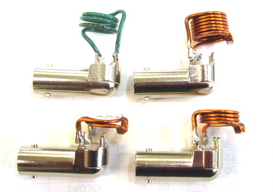
Figure: Four Candidate Pick-Up Coils. Top-Left self-wound 160-nH. Top-Right, surface-mount 257-nH from Coilcraft. Bottom-Left, 33 nH. Bottom-Right, 110 nH. All are soldered to a right-angle BNC socket.
We mount the coils over a conducting plane of carbon film. We connect them to a 3-dB attenuator and an Active Antenna Combiner (A3021B) acting as an amplifier to raise our signal to noise ratio before applying to the RF input of our Spectrometer (A3008B). We calibrate the combination of A3021B and A3008C so as to obtain accurate absolute power measurements for the pick-up coil and attenuator combination.
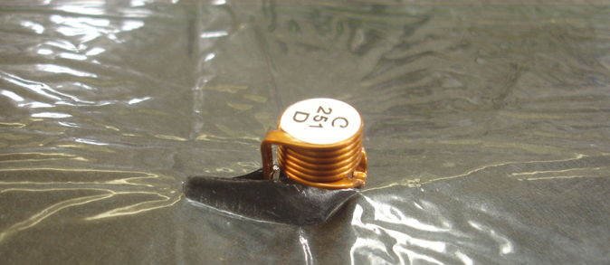
Figure: Pick-Up Coil on Reflecting Surface.
We have an A3028E transmitter on the end of a stick. We rotate it just above the pick-up coil and measure the received power with the help of the Spectrometer Tool and a Tcl script. When we have one hundred power measurements, we stop. We laterally 8 cm and repeat. We do the same for all four coils.
Figure: Received Power for Various Coils with Transmitter Rotating at Two Ranges.
Our home-made 160-nH coil picks up at least 5 dB more power than any other coil. Our concern is not with the absolute power received, but rather the change in power received when moving from range 0 cm to 8 cm. The average difference between the 0 cm and 8 cm ranges is 12 dB for the 160-nH coil, 9 dB for the 257-nH coil, and in-between for the other two. The ideal pick-up coil would always pick up more power from a transmitter at range 0 cm than one at 8 cm regardless of orientation. The standard deviation of the received power is for all coils around 6 dB. Assuming a normal distribution of received power with orientation, and assuming the effect of orientation is independent for coils at 0 cm and 8 cm, the likelihood of the coil at 8 cm receiving more power than the coil at 0 cm is 13% for the 160-nH coil, rising to 32% for the 257-nH coil. When we examine the power measurements, however, we see that the maximum power received for the 257-nH coil is only 5 dB higher than the average, while the minimum is 26 dB below the average.
We repeat our measurement for the 257-nH coil, this time recording all one hundred power measurements. We reject any measurements more than two standard deviations from the mean. We reject roughly 5% of measurements at both ranges. We examine the distribution of the remaining measurements. The average power at 0 cm is 7 dB higher than at 8 cm. The standard deviation of the power at 0 cm is 3.9 dB and at 8 cm is 2.1 dB. The standard deviation of the difference, assuming a normal distribution, is 4.4 dB. The probability of 0 cm receiving less power than 8 cm is 8%. Allowing for more errors due to the 5% extraordinary measurements, we estimate that a transmitter on top of one coil will be deemed to be closer to that coil than one 8 cm away 90% of the time. When we measure at 16 cm, the average power is 22 dB lower than at 0 cm, with standard deviation 1 dB. There is no chance we will confuse 16 cm and 0 cm.
As we rotate the transmitter directly over a coil, and we arrive at a rotation that yields an extraordinarily low power reception, we note that it is almost impossible to hold the transmitter in this location by hand. The slightest movement of the transmitter results in the power rising to a value within one standard deviation of the average. When a transmitter is implanted in a moving animal, the ALT's measurements of location from one transmitter sample to the next will have some degree of independence, so that by taking the average of these measurements over a hundred samples, we will be able to improve the precision of our location measurement, if not by a factor of ten, then by a factor of four.
We repeat some of these experiments with electrically conducting sheet in a plane over the coil. The received power drops by 10 dB, and standard deviation appears to remain close to 6 dB, before rejecting unusual measurements. We place conducting sheet between the transmitter and coil at range 8 cm. We see 10 dB less power and 6 dB standard deviation.
We have the following measurements of an IVC mouse cage from Pishan at ION.
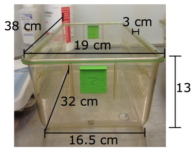
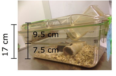
Figure: Dimensions of an IVC Mouse Cage.
From these, we decide to make the ALT platform 34 cm × 18 cm, with fifteen coils on an 8-cm grid extending 32 cm × 16 cm. Pishan also measures the space available between cages in an IVC rack.
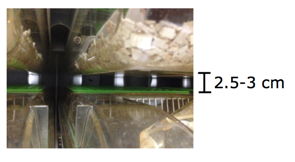
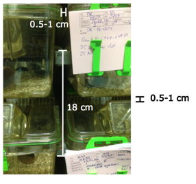
Figure: Dimensions of an IVC Mouse Cage.
If we remove the cage below, we have plenty of room for the height of our tracking platform. If we replace the water bottle with one that terminates 1 cm lower, we have space between the cages of at least 2.5 cm. We plan an ALT platform that allows 11 mm for coils and connectors on the top side, 3.5 mm for a plexiglass cover supported by standoffs, 3 mm spacing beneath the circuit board, and another 1.5 mm for an aluminum base with screws, making a total height of just under 20 mm.
With the 8-cm grid, our measurements suggest that the absolute maximum error we can make in a single-sample location measurement will be 8 cm. Given that these errors will occur less than 10% of the time, and we will be taking hundredds of partially-independent measurements per second, we believe we can reduce our measurement error by taking averages and increasing the measurement period until we are satisfied.
Development
2016
[24-JUN-16] We receive two A303201A printed circuit boards. We load the LWDAQ socket and the buck converters. We get 3V0 = 3.0 V and 3V3 = 3.5 V. We load amplifiers, power meter, and ADC into detector No8. Current consumption is now 36 mA from +5V. We attach a ×10 probe to PW8, the output of LT5534 power detector No8, on U0803-3, see S3032_1. Our pick-up coil, L0801, is a Coilcraft 2014VS-251. We place the antenna of an A3028E transmitter with cut-off leads on the coil. We see the following trace on the oscilloscope.
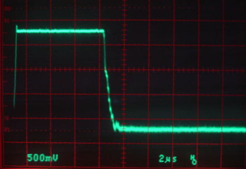
Figure: Detected Power for a 7-μs SCT Burst. Vertical 0.5 V/div, horizontal 2 μs/div. Burst power level is 2.3 V. Background is 0.3 V.
The plot below shows the response of the LT5534 to 900-MHz with a 3.0-V power supply. Using the plot, it appears that the power at the input of U0803 is −5 dBm during the SCT burst and −55 dBm otherwise.
Figure: Response of LT5534 to RF Input Power.
When our ambient 926-MHz interference is present, we see the following detected power. The interference produces a 0.6-V output, which implies an input power of −45 dBm.
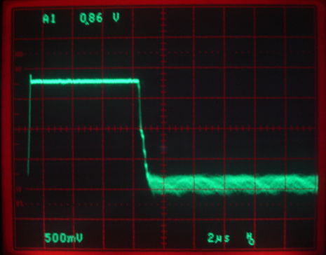
Figure: Detected Power for a 7-μs SCT Burst with Interference. Vertical 0.5 V/div, horizontal 2 μs/div. Burst power level is 2.3 V. Background is 0.6 V.
Our pick-up coil is paired with a 3-dB attenuator, R0801 in this case, which damps its response to 900 MHz so that the coil does not resonate. When the coil does not resonate, it is more omnidirectional in its response. The output of the attenuator we call A8. With the 257-nH coil, we expect to pick up around −40 dBm with the antenna of our SCT on the coil. The amplifier U0801 is a UPC2746 with gain 18 dB at 1 GHz. After U0801 the RF signal passes through a 100 pF capacitor and into another 3 dB attenuator R0802. The purpose of R0802 is to stabilize the amplifier at frequencies outside the pass-band of L0802, a B3588 902-928 MHz SAW filter. Within its pass-band, L0802 has impedance close to 50 Ω and insertion loss of 3 dB. But outside its pass-band its impedance is unspecified, and the UPC2746 will oscillate at such frequencies when improperly terminated. Beyond L0802 we have another attenuator to stabilize the next amplifier, U0802. The gain from A8 to RF8 is nominally 27 dB. Working backwards, it looks like A8 is −32 dBm when the antenna is on the coil.
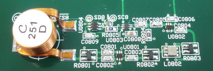
Figure: Power Detector No8. The RF signal path is from the lower left, R0801, anti-clockwise to C0807. The power detector chip is U0803. The ADC is U0804. Gain from the coil to the power detector is nominally 27 dB.
We place a transmitter on a frame cut from a paper cup and move it from the location of L0201 to L1301 in 4-cm steps (half-grid steps) within a faraday enclosure to block our interference.
Figure: Power Detect Voltage (PW) versus Position for 257-nH Pick-Up Coil.
At 0 cm, PW is 1.5 V, implying −27 dBm at the input of the power detector, and −54 dBm at A8. Our average for all orientations at 0 cm range for this pick-up coil was −57 dBm. If we were to operate outside a faraday enclosure, we could apply a threshold of 0.8 V to eliminate our ambient interference, and we would be left with detection from transmitters at ranges 8 cm and less for this particular orientation.
[01-JUL-16] We establish communication via USB cable from an Octal Data Receiver Y2 output. Our USBB-RA pinout is incorrect. We cut tracks and re-route the USB signals. We speed up the immediate sample transmission of P302701A07 so the bit period is 50 ns and have no trouble receiving at the A3032A.
[03-JUL-16] We transmit 40 MHz without corruption over a 1-m USB cable from an A3027E to our A3032A. Polarity of logic is correct. Delay from A3027E Y1O to A3032A TP1 is 15 ns.
[15-JUL-16] We have P3032X01 for the A3032A combined with the P302701A08 for the A3027E. The A3027E sends incoming notifications, most data messages, and all clock messages to the A3032, which stores them in RAM as four-byte messages. We can download from the A3032 just as if it were an A3027. With four A3028Es active, we get 98% of message in the A3032 compared to 99.5% in the A3027. The timestamps are stored in an identical manner, thus demonstrating that we have perfect synchronization between the Data Receiver and Animal Tracker.
[05-AUG-16] We are working on P3032X02. We have !CS8 (chip select for power detector eight) asserted after the A3032 receives an incoming notification.
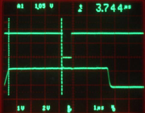
Figure: Power Detect Voltage (PW) and Chip Select (!CS8). We have a transmitter on the detector coil and a message decoding antenna nearby.
The delay between the start of the radio frequency burst and the assertion of CS8 is 3.7 μs. We now consult the data sheet of our eight-bit ADC, ADC081S101. We generate a clock signal at 20 MHz to transfer the eight ADC bits into our firmware. When we receive a data transmission, the A3032 stores the digitized power measurement in place of the message data. The top byte stored is the power measurement, the bottom byte is all zeros. Now move our transmitter around on a decoding antenna while displaying the digitized power measurement in the Receiver Instrument. We record our power signal to an archive and display with the Neuroarchiver.
Figure: Transmitter Power with Movement, Eight-Second Interval. A transmitter No4 rests upon an A3015C loop antenna. We move the antenna around over our power detector coil. For the first second, we see background power. For the next four seconds, we are moving from −30 cm to +30 cm over the coil. For the next three seconds we are moving more rapidly along the same path.
When the transmitter is within a few centimeters of the coil, power increases as we come closer. When the transmitter is roughly 8 cm from the coil, its power reaches a local minimum. We turn on three transmitters, place them in a beaker of water on the decoder antenna and move over the detector coil.
Figure: Transmitter Power with Movement, Eight-Second Interval. Three transmitters on a loop antenna. We move the transmitters from −30 cm to + 30 cm during the interval.
In the figure above, No2 has a simple peak in received power. But No1 and No4 show local minima due to destructive interference at the pick-up coil.
[09-AUG-08] We download power measurements from the A3032A with newly-upgraded A3027E P0245 and two transmitters. We occasionally see the timestamp signal turning into a full-scale square wave, at which point the Receiver Instrument resets the A3032A announcing it has encountered corrupted data. There is no corruption of the transmitter power measurements. We suspect that reception of the 20 MBPS serial message notification signal using a 40-MHz clock is unreliable.
[19-AUG-08] We observe intermittent, catastrophic corruption of the data stored in the A3032A memory. We study the de-serialization process with the help of a simulation of a 32-bit reception (for details and the simulation see here). With the correct design, we still see the intermittent corruption.
Figure: De-Serialization. The top signal is TXI. The next is CK. The next two are TXI synchronized with CK and !CK. The black lines are the TXI sample points. We have CK period 50 units so that 2 units would be 1 ns to simulate a 40-MHz clock. Here the sampling delay is 25 units, or 12.5 ns, which represents the delay between the falling edge of CK and the rising edge of CK.
The corruption always begins with a message of ID = 255 and contents 0xFFFFFFFF (eight-bit ID, sixteen-bit data, and eight-bit timestamp are all ones). Occasional reception notifications are being confused for clock transmissions. After we receive a data transmission notification, the A3032A takes time to store the data in RAM. The reception notification can begin before the A3032A is ready to receive. We could fix this in the A3027E firmware FV=8, but we have already shipped an A3027E with the existing firmware, so we resolve to fix the problem in the A3032A firmware. We forbid the A3032A from storing any data transmission with ID = 255. The corruption stops.
We now note the following erroneous power measurements, in which channel No2 receives the same measurement as No4. We have five transmitters running on one A3015C loop antenna over the A3032A pick-up coil.
Figure: Consecutive Message Confusion: Power Measurements Crossing No4 to No2.
Here are the raw message contents from the Neuroarchiver. The No4 and No5 messages are received consecutively, but they both have the same power measurement.
 index id value time  hex
   74   1 18432 154 $0148009A
   75   4 29440 156 $0473009C
   76   2 29440 156 $0273009C
   77  13 34048 193 $0D8500C1
   78   5 31488 221 $057B00DD
   79   1 18432 223 $014800DF
   80   4 29184 229 $047200E5
   81   2 29184 229 $027200E5
   82  13 34048 250 $0D8500FA
The No4 and No2 transmissions occur in the same 30-μs window. The reception notification for No2 is blocked by the data transmission of No4. The data transmission of No2 takes place, but the A3032A has not converted the antenna power, and so uses the previous antenna power, that of No4. We introduce the PMV (Power Measurement Valid) flag, which expires in 7.5 μs. Each power measurement is now valid only for one data transmission, and only if the data transmission occurs immediately after the measurement.
[20-AUG-16] We find more power measurement errors in our A3032A recordings. Here is the raw data for an error in which the No5 sample receives the No4 power measurement, while the No4 sample itself is missing.
 index id value time  hex   68  13 33792 162 $0D8400A2
   69   1 18176 166 $014700A6
   70   4 29184 175 $047200AF
   71   5 31744 181 $057C00B5
   72   2 36864 184 $029000B8
   73   1 18688 228 $014900E4
   74  13 34048 234 $0D8500EA
   75   5 29184 236 $057200EC
   76   2 37120 240 $029100F0
   77   0  3506  38 $000DB226
   78   1 18432  35 $01480023
   79   4 29184  39 $04720027
These errors arise in the following way. The No4 message reception begins and the A3032A receives an incoming notification. The A3032A converts the No4 incoming power. Within a few microseconds, however, the No4 message reception is corrupted and aborted by the No5 message transmission. The No5 transmission is powerful enough that it is successful. By the time the incoming notification is complete, the No5 message reception is well underway, and no incoming notification is transmitted by the A3027E. At the end of the No5 message reception, the A3027E sends a data transmission notification and the A3032A stores the No4 power measurement as a No5 measurement. The A3032A has no record of the aborted No4 message.
[23-AUG-16] We modify the P302702A09 firmware so that the message detectors refrain from asserting their RCV flags until they have received sixteen bits of message data, rather than only eight as before.
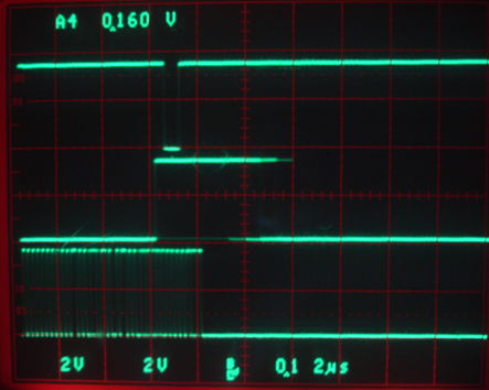
Figure: Chip Select (!CS8, Top), Message Incoming (MSGI, Center) and Transmit Output (TXO, Bottom). We have one dual-channel A3028A transmitter on the detector coil and a message decoding antenna nearby. We are triggering on TXO.
Transmission bursts vary in length from 36 × 195 ns = 7.0 μs to 36 × 215 ns = 7.7 μs. The transmission burst shown above is 7.7 μs. The power measurement is complete 6.8 μs after the start of the burst. A shorter burst will have its power measurement begin sooner, but in any case we are certain that the power measurement will be complete at least 0.2 μs before the end of the burst. With no transmitter turned on, the background rate of incoming notifications is less than one per ten seconds. When we go back to requiring only eight bits before we issue an incoming notification, our background rate is higher than ten per second.
The notifications are still 33 × 50 ns = 1650 ns long. The incoming notification ends 1.1 μs before the data notification begins. Data storage in the A3032 is complete 5.5 μs after the rising edge of MSGI and 5.1 μs after the rising edge of PMV. We reduce the PMV assertion time from 7.5 μs to 5.2 μs.
In P302702A09 we alter the Message Notifier so that it commences a clock or data notification only when the RAM Controller stores a byte on a four-byte boundary. This prevents a data notification from using a previous message's ID, which would otherwise assign the wrong ID to the most recent power measurement in the A3032A.
With one decoding antenna and four transmitters running, we see one or two glitches per second in the raw data displayed in the Receiver Instrument. In the Neuroarchiver, after signal reconstruction, we see one or two every ten seconds. With the glitch threshold set to 1000 we see no glitches in one hundred seconds. The glitches take the form of a jump up or down to the power measurement of another transmitter. When we look at the raw transmitter messages from the A3027E, we see similar glitches, so we assume they are bad messages caused by collisions.
[26-AUG-16] We run four transmitters on our receive antenna, No2, No4, No5, and No13. We note bad messages on channel No2 in particular, but also in the others. In one 1-s interval, No2 has 515 samples and No13 has 504, while the others have 512 and 511. These bad message on No2 stop when we remove the other three transmitters from the antenna. The bad messages are messages from other transmitters that have been corrupted so as to appear to be messages from No2. When the A3032A receives the bad message, it takes a fresh and accurate power measurement for the transmitter that generated the message, and stores this valid measurement with an invalide channel number.
In P3032X04 we add serial interfaces for all fifteen detector coils. The firmware now occupies 362 logic cells of 512 available. Each detector uses 10 logic cells. The detector readout proceeds as follows. First, all ADCs are read out in parallel by a common serial clock. The eight bits of each ADC result are shifted into an eight-bit register. When we store the fifteen bytes, we store the first detector byte repeatedly, and shift the the bytes from register 15 to register 1 as we do so.
Our four transmitters are on the A3032A within a faraday enclosure with two pick-up antennas. The standard deviation of the power measurements is around 400 counts rms. We note that one ADC count appears as 256 counts in our display. We add 100 pF from PWR to 0V. Noise drops to 250 counts rms. We add 1 nF and we see more small spikes on the data, so that total noise rises to 300 counts rms.
We load parts into detectors 7 and 9, with a 33 nH inductor for No9 and 150 nH in No7. We move a transmitter on a glass rod over the three sizes of coil and observe the power measurement. All three coils are working.
[30-AUG-16] We have two transmitters No2 and No4 on a single glass rod with their antenna loops at 90° to one another. We place the A3032A inside a faraday enclosure with two receiver antennas. We move them from far to the left, over the 257-nH coil, and to the right. We repeat with a different orientation of the glass rod. We obtain the following traces for power.
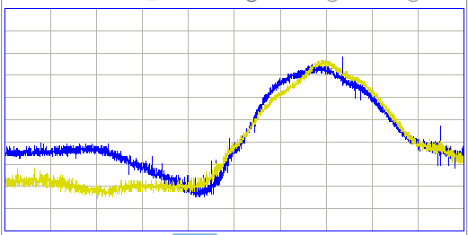
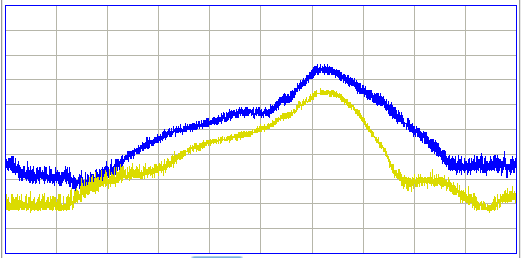
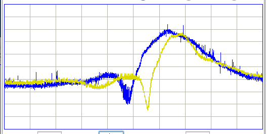
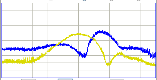
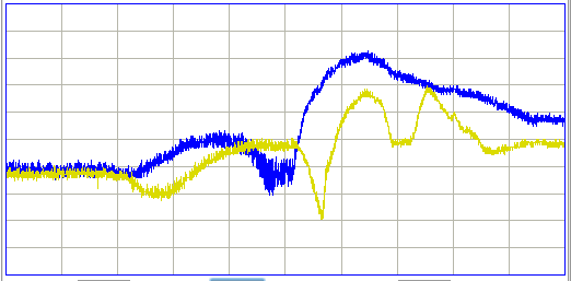
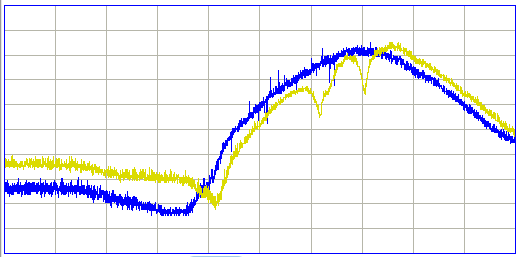
Figure: Power Traces while Traversing 257 nH Coil at Center of A3032A. The two transmitters are directly over the coil half-way through each sweep. The range is 0-40,000 counts.
The 257-nH coil is in Detector 8, in the center of the circuit board. For certain orientations, we see minima in power reception when the transmitter is directly over the coil. Such minima will disturb our position measurement. We try with the 33-nH coil installed at the edge of the circuit board in Detector 9.
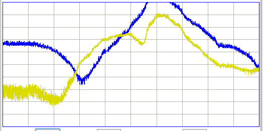
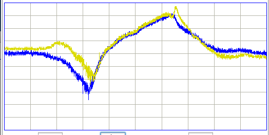
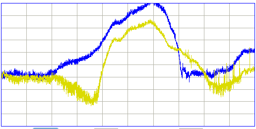
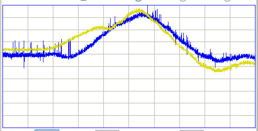
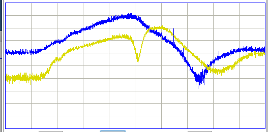
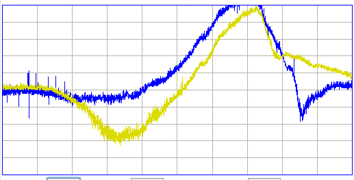
Figure: Power Traces while Traversing 33 nH Coil at Edge of A3032A. The two transmitters are directly over the coil half-way through each sweep. The range is 0-40,000 counts. The 33-nH coil is more sensitive to 915 MHz, and occasionally the trace rises above the top of the plots.
We hold the two transmitters directly over each of our three detector coils and rotate them on their glass rod for eight seconds.
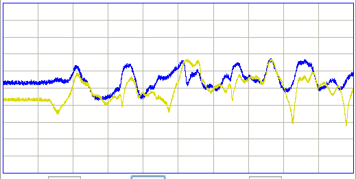
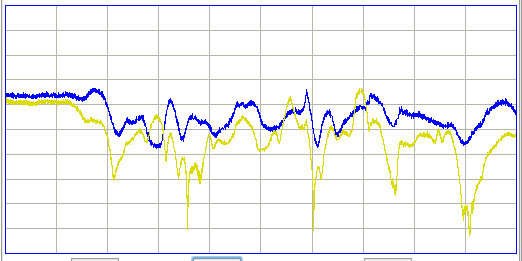
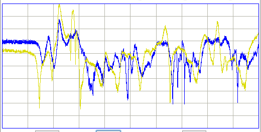
Figure: Power Traces while Rotating over Three Coils. Left: 33 nH in Detector 9 at board edge, Center: 108 nH in Detector 7 at board edge, Right: 257 nH in Detector 8 at board center. The scale for the left and center is 0-65,000 counts. For the right is 0-40,000 counts.
We repeat our 8-s rotation recording several times for the 33 nH and 257 nH coils. We obtain similar results. We see only one spike down to background power with the 33 nH inductor, and dozens with the 257 nH. We replace the 108 nH and 257 nH coils with 33 nH coils. We repeat our rotation experiment with the new 33 nH coil in the center of the circuit board.
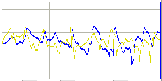
Figure: Power Traces while Rotating over Central 33-nH Coil. Scale is 0-65,000 counts.
We see similar behavior from the 33 nH coil as we did previously from the 257 nH coil in the same location. We conclude that the coil inductance has little to do with the performance of the power detector. We will use the 33 nH inductor because it has a greater maximum power.
We set up a prototype Locator Instrument with a new lwdaq_locator analysis based upon the lwdaq_receiver routine. We modify the P3032X04 firmware so it stores the power from Detectors 8 and 9. We take the weighted centroid of these and plot it versus time on the Locator screen. We move two transmitters back and forth from one coil to the other.
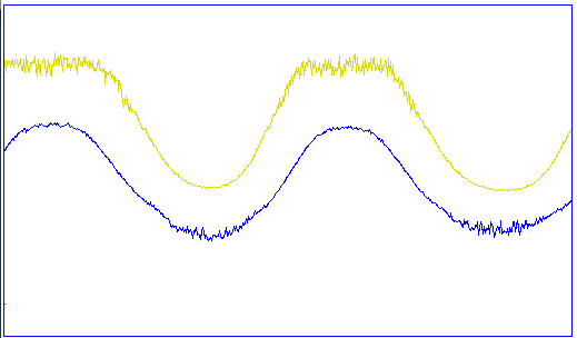
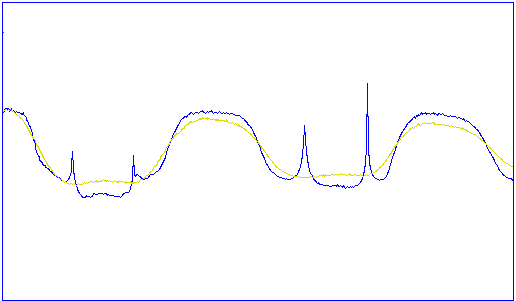
Figure: Location Traces. Upwards is towards the edge of the circuit board, from Detector 8 to 9. Left: A typical response. Right: For some orientations, we see spikes in calculated position.
The spikes in calculated position are caused by a drop in power received by the center coil. The transmitter appears to jump to the left when the power received by the center coil spikes downwards.
[13-SEP-16] We load the remaining detector coils and amplifiers onto our prototype A3032A.
[14-SEP-16] We have modified the Receiver Instrument in LWDAQ 8.4.3 so that it opens a socket and closes the socket every time it downloads a block of data from the LWDAQ Driver, rather than keeping the socket open until it has received all the blocks it needs. By closing the socket, the Receiver Instrument allows another LWDAQ process to connect to the same LWDAQ Driver and download from another device. In this way, we are able to download from two A3027E and one A3032A without getting more than half a second behind in either recording after ten minutes.
We place a transmitter on each of the fifteen coils in turn. We observe the pulse Un03-3 during the transmitter bursts. We correct a few soldering errors. We now have 2.4-V pulses on all fifteen detectors when the transmitter is resting on the detector coil. Firmware P3032X05.abl stores the SCT channel number, sample value, and timestamp of all messages it receives from the A3027E, plus the fifteen power measurements and its own firmware version number. We reset the A3032A and download 20 bytes with the Terminal Instrument to examine the digitized power measurements. With the transmitter resting on the detector coil we get power 167-173 counts on all coils. The maximum power on any other coil is <140 counts, and usually <120 counts. With the transmitter isolated from the A3032A by a faraday enclosure, we get between 50 and 90 counts in a single measurement. With a probe on the power voltage, we see variation from 0.4-0.9 V from our local interference.
[16-SEP-16] The Neuroarchiver now calculates the position of a transmitter on the array of fifteen coils. We subtract a threshold from the power measurements. Any coil that detects power above the threshold takes part in the weighted centroid calculation of the transmitter position. We square the power above threshold, or net power, and multiply by the coil's position in x and y, then divide at the end by the sum of squared net powers. We have a plastic platform above the coil array, its surface 15 mm above the surface of the circuit board. The origin is the center of coil number one, and x is along the long side of the grid. We place a transmitter in a beaker with 40 ml of water and set it on the platform in various places. The standard deviation of position when untouched, with the faraday enclosure door shut, each measurement an average over half a second, is 0.5 mm. We move the beaker in 1-cm steps a total of 28 cm in a straight line close to the long axis of the array. We plot the measured position at each point.
Figure: Tracker Measurement of Position While Moving in Straight Line. The center of the transmitter and its antenna moves approximately from (2 cm, 10 cm) to to (30 cm, 10 cm). The power threshold is 80 counts. We are taking the average position over 4-s intervals, but standard deviation over 0.5-s intervals is only 0.5 mm. Data in archive M1474062026.ndf.
The following plot shows how the tracker measurements vary with actual position. The stage is the piece of paper with one-centimeter graduations along which we move the transmitter in its beaker of water.
Figure: Tracker-Measured X ad Y with Stage Position. The stage is parallel to the x axis of the tracker. The center of the transmitter and its antenna moves approximately from (2 cm, 10 cm) to to (30 cm, 10 cm). The power threshold is 80 counts. We are taking the average position over 4-s intervals. The standard deviation over 0.5-s intervals is only 0.5 mm.
Our absolute accuracy in measuring animal position will be no better than one or two centimeters, but our relative accuracy will be a few millimeters in most places, and our resolution will be a fraction of a millimater.
[17-SEP-16] Neuroarchiver 113 now provides a prototype Tracker Window, run by the Neurotracker routines. In the window, we plot the A3032A location measurements during each playback interval. Each power measurement gets its own point, and a line to the next power measurement. A 512 SPS transmitter receivers 512 points per second in the plot.
Figure: Tracker Window for 32-s Interval. Horizontal is x, 0-32 cm and vertical is y 0-16 cm. During this interval, we pick up and move the transmitter from 28 cm to 0 cm on our stage.
The Neuroarchiver permits us to vary not only the threshold for net power, but also the exponent we apply to the net power in the weighted centroid calculation of location. When re-playing archive M1474062026 of our translation experiment, we find that an exponent of 1.0 reduces the spikes in y-coordinate that occur when we move directly over the center-line coils.
[20-SEP-16] We add to the P3032X01 firmware calibration constants for all fifteen coils. We place the A3032A in a faraday enclosure with a transmitter on the outside, so we record the noise power output for the detectors. In the Neuroarchiver, we take the string with the background powers and put it into the following Toolmaker script to obtain the lines required by the firmware.
set l "29.8 30.3 29.6 44.6 29.1 38.8 37.7 23.3 22.0 25.5 25.8 40.6 26.4 28.3 23.5"
set i 1
foreach a $l {
  LWDAQ_print $t "  p$i\_calib = [expr round($a)+1]\;"
  incr i
}
The A3032A now stores these background powers after its timestamp messages, so the Neurotracker can read them from a clock message, subtract them from the detector coil measurements, and so remove the effect of gain variation between the detector amplifiers. The spread of amplifier gain is 24-45 ADC counts, or 0.31-0.58 V, which the LT5534 typical response plot suggests is −55 dBm to −47 dBm. We expect thermal noise of −93 dB at the coil for 900-930 MHz, which we apply to 3-dB attenuator and a UPC2746 with noise figure 6 dB. Our effective input noise is −84 dBm. With 27 dB of gain, the noise should be −57 dBm at the power detector. The LT5534 also has an output offset of 0-300 mV. The variation in our background power levels could be due to either gain difference or variation in offset.
[23-SEP-16] The Neurotracker window now show the average position of each transmitter channel as a dot on the screen. With the "path" button we can turn on plotting of all location measurements in the interval. We have enhanced the glitch filter so it operates upon two-dimensional data, and rejects aberrations greater than ten times the glitch filter under all circumstances. The glitch filter now eliminates most bad power measurements created by collisions.
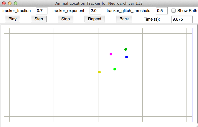
Figure: Neurotracker Window. Five transmitters in a 50-ml beaker. Dots show the average position of devices during the 1/16-s interval.
We place five A3028E transmitters in a 50-ml beaker of water. They are piled up one upon the other up to a heigh of 3 cm. We place the beaker on our tracking platform and move it around at random, rotating as we go, but allowing the beaker edge to get no closer than 2 cm to the edge. We record the tracker measurements and play back in 1/16-s intervals. The following processor line saves the average positions to disk.
append result "$info(tracker_average_x) $info(tracker_average_y) "
For various values of threshold fraction and exponent we calculate the average and standard deviation of the separation of four pairs of transmitters selected from the five in the beaker.
Threshold
Fraction |
Exponent |
Average
Separation (cm) |
Stdev
Separation (cm) |
| 0.7 | 2.0 | 3.0 | 2.1 |
| 0.5 | 2.0 | 2.7 | 1.6 |
| 0.5 | 1.0 | 2.9 | 1.8 |
| 0.7 | 1.0 | 2.8 | 1.8 |
Table: Relative Tracking Accuracy for Threshold Fraction and Exponent. Using 0-40 s of archive M1474657863, four pairs of transmitters chosen for separation calculation.
The performance of the tracker appears to be only weakly dependent upon the threshold fraction and exponent, but 0.5 and 2.0 give the best results.
[27-SEP-16] We abandon the power calibration stored in the A3032A clock messages after we find that the detector output for more powerful signals is more reliable without the calibration adjustment. It appears that the difference in background power level in the coils is due to variations in noise rather than gain. Instead of using all coils to calculate position, we use only those within a centroid extent, which we can set in the Neurotracker window. We place seven transmitters in a 500-ml beaker. No3/4 is a dual-channel A3028D. All others are A3028E. We translate the beaker all over the platform, varying height from 0-50 mm, but not rotating. We place the beaker on the platform and rotate in place in several locations. We record coil powers in M1475011404.
| Extent (cm) |
Fraction |
Exponent |
Glitch (cm) |
Average
Spread (cm) |
Stdev
Spread (cm) |
| 12 | 0.3 | 1.0 | 0.1 | 5.5 | 3.8 |
| 12 | 0.3 | 1.0 | 0.5 | 5.4 | 3.6 |
| 12 | 0.5 | 1.0 | 0.5 | 5.8 | 3.7 |
| 20 | 0.5 | 1.0 | 0.5 | 5.0 | 2.9 |
| 100 | 0.5 | 1.0 | 0.5 | 5.7 | 2.6 |
| 8 | 0.5 | 1.0 | 0.5 | 7.1 | 5.7 |
| 12 | 0.5 | 2.0 | 0.5 | 6.2 | 3.9 |
| 12 | 0.7 | 2.0 | 0.5 | 6.6 | 4.5 |
Table: Relative Tracking Accuracy for Extent, Fraction, and Exponent. Using 0-89 s of archive M1475011404 we calculate the spread in x-coordinate in every 1/16-s interval.
When the extent is 8 cm, all transmitters are located on the coil with the maximum detected power. When the extent is 100 cm, we use all coils. Although the standard deviation of the spread is at its lowest, the position of the transmitters tends to be drawn towards the center of the platform. We get better reporting of the actual position of the beaker full of transmitters with an extent of 12 cm, threshold 0.3, and exponent 1.0.
When two transmitters collide, we can still receive the message from one of them, but we will get the power from both, so the resulting location is somewhere between the two transmitters. A glitch threshold of 0.1 cm eliminates almost all jumps in location caused by collisions between transmitters.
We looked at the separation of six pairs taken from the seven transmitters and calculated the standard deviation of their separation during the period when we were not rotating the beaker. When we rotate the beaker, the transmitters move around. We obtain a standard deviation of 1.9 cm.
[30-SEP-16] We place an A3028E transmitter with 15-cm leads on the platform with its body centered on position (0,0) cm. We coil the leads over the body. The tracker measures position (0.6,1.9) cm. We lay the leads straight out along the line x = 0 cm. The tracker measures position (0.2,7.5) cm.
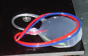
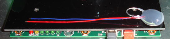
Figure: Transmitter Leads Coiled and Straight. When we straighten the 15-cm leads, the measured transmitter position moves by 5.6 cm along the direction of the leads.
The leads transmit signal power also, because they are part of the high-frequency ground of the antenna. The center of the transmitter is the center of its power emission, and so moves as the leads move.
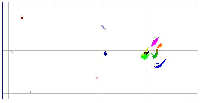
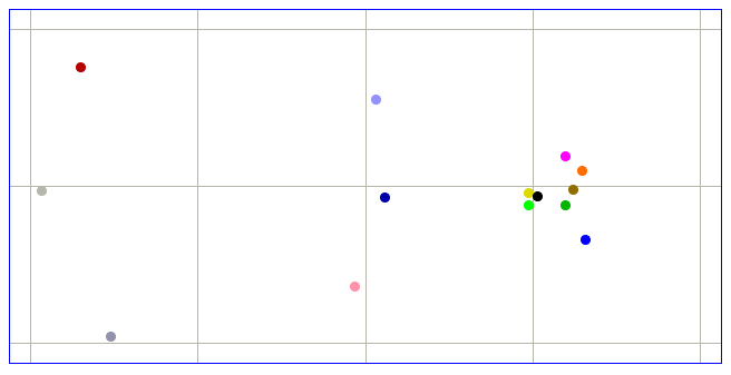
Figure: Fourteen Transmitters on the Platform. Left: paths for one-second interval. Right: average positions for one-second interval. Archive M1475253453 recorded with firmware version P3032X05. We use extent = 12 cm, threshold = 0.3, exponent = 1.0.
We put fourteen transmitters on the platform. Numbers 10, 11, 12 are A3028E with 15-cm leads in their shipping bags, and located over coils 1, 2, and 3 respectively. No 7, and 8 are A3028E with short leads over coils 7 and 9. No14 is A3028B with 4.5-cm leads over coil 8. The remainder are A3028E in a beaker approximately over coil 10.
[04-OCT-16] We attach serial number V0383 to our first A3032A. We have completed a second circuit, V0384, and a third is on its way, which will be V0385.
[05-OCT-16] Firmware version P3032X06 replaces power calibration in the clock messages with the location of each coil described as two four-bit numbers. The sixteen payload bytes are now "0 1 2 16 17 18 32 33 34 48 49 50 64 65 66 6". The last one is the firmware version. the first is the location of the first coil (0,0) in units of grid spacing, which for the A3032A is 8 cm. The final coil is 66, which is (4,2), or (32 cm, 8 cm). The Neurotracker works in units of coil spacing, and does not need to know what the actual spacing is in order to plot position on a grid.
Firmware P3032A01 will be our first production release firmware. We enhance the grid encoding in the following way. We assume the first coil will always have coordinate (0,0), so we write into its coordinates the grid spacing in centimeters. The remaining coils have their coordinates in grid spacing units. The final number is an encoding version number, one (1) in this case, to indicate how the coil locations are encoded. Instead of writing the Octal Data Receiver firmware version number into the clock messages, we write the A3032 firmware version number, on the grounds that the Octal Data Receiver firmware version is available from the Octal Data Receiver directly.
[11-OCT-16] Here is an example message print-out from the Neuroarchiver.
Data Recorder Firmware Version 6.
Total 1113 messages, 128 clocks, 0 errors, and 0 null messages.
Messages 0 to 10 (index id value timestamp $hex):
    0   0 49787   6 $00C27B06 08010210111220212230313240414201
    1   3 44287  52 $03ACFF34 94824D71675A675757503D3738563D06
    2   4 44031  84 $04ABFF54 93814D706659655655503A363A543A06
    3   3 44072 116 $03AC2874 97855271685B6959564B423A3F554106
    4   4 43883 137 $04AB6B89 95834F6F675D6959595145383D583F06
    5   3 44067 170 $03AC23AA 94834E6F685D6958584943413A574106
    6   4 43846 198 $04AB46C6 94824E70675A675655513C353A553806
    7   3 44087 232 $03AC37E8 94824E6F675B6856554E3D3A38553906
    8   0 49788   6 $00C27C06 08010210111220212230313240414201
    9   4 43874  16 $04AB6210 94824E70665A675758513F3739573F06
   10   3 44220  38 $03ACBC26 93824E6F675C68585850403B3A573C06
End of Messages
We ship to ION/UCL A3032A numbers V0383 and V0384, keeping V0385 for ourselves. Along with them we ship A3027E number Q0197 which we upgraded to A3027E with firmware version 9.
2017
[10-JAN-17] We have been examining an ALT archive, M1481291633.ndf, and accompanying overhead video of four mice in a cage on the ALT platform at ION/UCL. The platform is on a table-top with no faraday enclosure. Three antennas are placed around the edges of the cage. Two of the mice have dual-channel A3028A transmitters implanted and the other two do not. The two mice with implanted transmitters have dental cement head fixtures that we can identify occasionally in the video recording. Reception is robust 80% of the time, but drops to 0% occasionally. The loss of reception causes large errors in the calculation of location. We introduce into Neurotracker a loss parameter. We set loss to 30, for which any interval with loss 30% or more will be given the same position as the previous interval. Signal loss now causes the tracker location to stop in one place, then jump to a new location when reception recovers.
The power measurements from one transmitter are often mixed with those of another, as a result of collisions between the two transmitters. Instead of taking all power samples in an interval and trying to remove the foreign power measurements before taking an average, we use the median power measurement, which is almost always reliable, because the number of collisions between the two transmitters is almost never going to be greater than 50%. The location measurement is far more stable after this modification.
After several hours looking at the video and tracking, we are convinced that the time synchronization between the two is correct to within a couple of seconds. We watch the mice moving around in the first ten minutes of the recording. When we use a subset of the detector coils to calculate position, such as is possible by setting the Neurotracker's extent to 12 cm, the transmitter location experiences occasional jumps of several centimeters that are not caused by signal loss. If we use all coils, we find that the calculated location is more stable, but moves several centimeters inwards from the left and right edges of the platform (x = 0 cm and x = 32 cm ends) as a result of the influence of coils far away in x upon the calculation of x.
We change the way we determine the power threshold that allows a detector to contribute to the location calculation. We now use the average detector power in place of the minimum power, so the threshold is fraction of the way from the average to the maximum detector power. We set the fraction to 0.0, using the average itself as the threshold, and extent to 100 to include all coils, and exponent to 1.0. We obtain stable and continuous location measurement.
During a period when all four mice are not moving, we record the position transmitter No7/8 for 64 s with intervals of 1/16 s so as to obtain 1024 intervals, each with two measurements of x and y. We obtain the following discrete Fourier transform of the four measurements.
Figure: Location Spectrum, 16 Sample per Second. The discrete Fourier transform of 64 seconds of x and y from each of the No7 and No8 channels of a single dual-channel transmitter.
We were hoping to see heartbeat and respiration in this transform, but we see no sign of any peak above 1 Hz.
We enhance the Neurotracker so it will show us the path taken by the transmitter in through previous intervals. We set the playback interval to 1 s and persistence to 2000 so as to display the path of both No7/8 and No13/14 transmitters during the first 2000 s of the recording.
Figure: Range of Measurement During Half an Hour, 1 Sample per Second. We have extent = 100 cm, fraction = 0.0, exponent = 1.0, loss = 30%, persistence = 2000.
According to overhead video, the No7/8 device (salmon and light blue) ranged at least x = 2-30 cm and y = 2-14 cm, visiting the top-left, bottom-left, and bottom-right corners. Transmitter No13/14 remained on the left side of the cage except for one trip around the water bottle spout at the center. The path recorded for each animal corresponds well to the nature of the movement and exploration by each animal, but the extent is compressed in the x-direction to a range of 20 cm when we observe at least 28 cm. We change the extent parameter to 16 cm, so that no coil more than 16 cm from the measured location will be used in the calculation (the calculation is iterative). We obtain the following half-hour paths.
Figure: Range of Measurement During Half an Hour, 1 Sample per Second. As above, but extent = 16 cm.
The range is increased in both x and y, but we note the degeneration of the location calculation at the top and bottom sides, and it is not clear that the left-most excursion of the No13/14 transmitter is real or artifact of calculation. We could scale the x measurement so as to stretch it out to the full width of the platform, but such a transformation could be applied just as easily later. So long as we have reception, the location measurement as it is now allows us to deduce when the animals are close to one another or far apart, when they are moving or stationary, and the direction in which they move.
We apply the same calculation to the location of a two-channel transmitter in a beaker of water within an FE2F faraday enclosure, as recorded in M1476195273. When we recorded this archive, we moved the transmitter along the length of the platform in x and increased y by 1 cm at each end. We obtain the following path with a 1/16-s playback interval.
Figure: Range of Measurement During Scan of Transmitter, 16 Samples per Second. Recorded in FE2F faraday enclosure. Parameters as above, but extent = 100 cm.
Here we know the actual range is 0-32 cm in x and 0-16 cm in y. We measure 4-28 cm in x and 3-16 cm in y. We see distortion of the paths by the measurement, in particular in the upper-center. We observe such distortions within Faraday enclosures, but not out in the open. The tracks demonstrated sufficient accuracy to determine proximity, movement, and direction.
[19-JAN-17] We have from ION half an hour of ALT recording from a transmitter No13/14 in a solitary, freely-moving mouse. We have overhead, color video showing the mouse's movements. The video recording has a timestamp in the top left corner during playback. We compare the video and the tracking for half a dozen key moments in the movement of the animal. The time in the video recording is 7 seconds behind the time of the NDF archive. We work with 0.25-s intervals and accept any interval with up to 50% loss. We reject roughly half the intervals because of loss, and there are stretches of several seconds in which we obtain no tracker location measurement.
We proceed through the ALT recording, using the new "*" value for the persistence parameter, so as to leave all tracks on the tracker map. The following figure shows the track of both the No13 and No14 channels for the entire half-hour recording.
Figure: Movement of Implanted Transmitter, 4 Samples per Second. Recorded out in the open with three antennas. ALT archive M1484767281.ndf. Green and blue lines are the tracks of the No13 and No14 channels. Black line is the rectangle of the cage as it appears in the distorted space of the tracker measurements. Red numbers are points of interest. We later realized that we were using threshold fraction 0.0 to obtain position, when we should have been using 0.3 or 0.5.
As we play through the tracker archive, we watch for times when we get several seconds of consecutive location measurements, and we check to see where the animal is during these periods. We soon find that point (1) in the figure corresponds to the top-left corner of the cage in the view of the camera, point (2) is top-right, point (3) is bottom-right, and point (4) is bottom-left. The animal spends several ten-second periods next to the water spout in the center of the cage, which is point (5). The location calculation is transforming the rectangle of the cage into the shape drawn in black. The transformation is conformal, in that it preserves angles locally, but distorts larger shapes. So long as all transmitters are implanted into the same side of an animal's body, with the antenna and body of the transmitter oriented the same way, we can expect the same conformal transformation of the cage rectangle for all animals.
Points (6) and (7) are interesting because they contain no position measurements. In the case of (6) it could be that the transmitter does enter this area, but the area is a reception dead spot, so we obtain no location measurements. We would still expect, however, for the tracks to cross this area. The mouse has its own habits of movement about the cage, and the transmitter is on its left side. We suspect that the transmitter never crosses area (6). In the case of area (7), we did not see the mouse moving along that wall from left to right with its left pressed against the wall, so the absence of tracks in region (7) may be genuine. A recording with more reliable reception would help us obtain a better understanding of such empty areas.
The three pick-up antennas for the Octal Data Receiver are close to the cage. These antennas resonate at the transmitter frequencies, and so affect the propagation of the transmitter radio wave power. We would rather have those antennas farther from the cage, but this would result in even poorer reception out in the open. Our next step is to obtain the same type of recording with the tracker platform at the center of a faraday enclosure with a substantial absorber in the ceiling, and the receiver antennas 10 cm from the platform edges.
[24-FEB-17] We receive from ION a recording from a dual-channel transmitter in one mouse in a cage in a faraday enclosure. There are two data antennas, but one is lying flat on the bottom of the cage, so reception is imperfect.
Figure: Reception versus Time for 2000-s Recording in Faraday Enclosure at ION.
We have video from the side of the cage for the entire period. During the periods of good reception, the animal is at times moving, stationary, and inactive. We examine the coil power measurements when the mouse is in known positions. The time of the archive and the video appears to be synchronized to within a second. At time 17:08:14, the animal is in the front-left corner of the cage facing the camera, with the transmitter on its right side, at roughly x = 1 cm and y = 4 cm. Median coil powers for a 1/16th second interval are: 90.0 86.0 78.0 81.0 70.0 65.0 86.0 61.0 83.0 81.0 32.0 41.0 26.0 79.0 68.0. We see that coil No7 receives power 86 counts, even though it is 20 cm fro the transmitter, while No2 receives 86 counts when it is 4 cm from the transmitter. We are unable to duplicate such coil measurements with a beaker of water and a transmitter. At time 17:08:45 the mouse rears up at x = 2 cm, y = 2 cm and coil powers are: 74.0 88.0 62.0 62.0 59.0 71.0 97.0 58.0 79.0 94.0 50.0 67.0 40.0 89.0 81.0. We receive maximum power in coil No7, which is 14 cm from the animal, and the second highest power in No10, which is 22 cm from the animal.
We attempt to duplicate these irregular power measurements with a transmitter in a beaker of water, which we translate back and forth over our ALT, and raise up above the ALT by several centimeters. In all cases, the power measurements decrease with range, and we do not see peaks of power in coils 20 cm away.
[07-MAR-17] We receive a recording of a transmitter in a beaker of water being moved along the line x = 0 cm in four steps, and then taken off the platform and set to one side. We have one recording for each of the two ALTs at ION/UCL. When the transmitter is off to the side, the coil power measurement remains significant and varied. We place a transmitter at the exact center of A3032A serial number V0385 inside an FE2F faraday enclosure. We measure coil powers 1-15. We take the transmitter out of the enclosure, place it on an antenna two meters away, and shut the enclosure. We measure coil power. We cover the transmitter with conducting sheet and open the enclosure. We measure coil power. We make the following plot.
Figure: Coil Power versus Coil Number.
When the transmitter is outside the enclosure, we receive none of its power at the detector coils. But we are still able to record the coil power values during each message transmission because we are receiving the messages with an antenna outside the enclosure. These power measurements tell us what the detector power will be in the absence of an message transmission, and we call them the background power measurements. When we open the enclosure, we allow our local −50 dBm 926-MHz interference into the enclosure to be received at the detector coils. We see little difference between the background with the door open or closed, which suggests that the background is dominated by an electrical offset in the output of each detector.
We subtract the background power from the power we obtain with the transmitter in the center of the enclosure to obtain the corrected power at each coil. The corrected power shows only two peaks: one in detector 8, directly beneath the transmitter, and the other under detector 11, 8 cm in the y-direction. The un-corrected power shows an additional peak on coil 4, 12 cm away from the transmitter, and the power in detectors 12 and 15 is significant.
Suppose we use the un-corrected plot to calculate location. The average power is 47 counts and the maximum is 144 counts. With threshold fraction 0.3, the threshold will be 47 + 0.3 × (144−47) = 76. Coil 8 will have net intensity 68 and coil 11 will have net intensity 5. If we use the corrected plot with the same threshold fraction we have coil 8 with net intensity 96 and coil 11 with 42. Furthermore, we could use a lower threshold and make more use of coils 7 and 9 as well, without bringing in background power form coil 15.
We implement background power subtraction in our lwdaq_locator routine, which powers the Neurotracker's location measurement. But we now find that the background power of coil No15 has dropped from 44 to 22. Using the latest background power, we obtain the following coil power measurements for a transmitter in a beaker of water.
Figure: Coil Power versus Coil Number. Three coils, No1, No8, and No15, with background power subtracted.
While editing the Neuroarchiver, we discover that we used threshold fraction 0.0 when analyzing the recordings of 12-JAN-17, 18-JAN-17 and 19-JAN-17. As a result, the measured locations do not extend the full length and breadth of the tracking platform, but are also less dependent upon individual coils, and therefore more stable with respect to small movements.
Further experimentation with the threshold fraction reveals that we obtain a less erratic measurement of position if we use an absolute value for the threshold, rather than calculating the threshold from the maximum and average coil powers. With threshold 60, background power subtraction, and extent 12 cm, we place the transmitter at the center of each square made by sets of four detector coils and rotate and raise and lower the beaker. The tracker measurement is within ±4 cm of the correct position 95% of the time, ±8 cm 99% of the time, but jumps away by 20 cm or more 1% of the time. If we can eliminate such jumps with a two-dimensional glitch filter, the tracker accuracy will be roughly 2 cm rms.
[15-MAR-17] We receive from ION/UCL background power recordings from both of their A3032A ALTs, and complimentary recordings with a transmitter sitting on the platform.
Figure: Background Power and Signal Power for ALT1 and ALT2 at ION. We do not know which serial number corresponds to ALT1 and ALT2, but one is V0384 and the other V0385.
The background power varies from 20-40 counts and appears to be independent from one ALT to the next. With the SCT inside, we get peak power around 150 counts and most coils pick up power around 80 counts. But for implanted transmitters, we get peak power as low as 120 counts with most coils picking up only 50 counts, at which point the 20-40 variation in background power starts to have a strong effect upon the measured position.
[27-MAR-17] Our LT5534 power detector is logarithmic over six orders of magnitude. Its typical response is 41 mV/dB with offset of 0-380 mV. We digitize the output with an ADC081S101 powered by 3.3 V. We expect 32 ADC counts to represent a factor of ten increase in detected power. The zero-power offset can be anything from 0-29 counts. In the 902-928 MHz band we expect thermal noise of 0.5 pW (−93 dBm) at the input to our detector amplifiers. Our UPC2746 amplifiers have a noise figure less than 5.5 dB, so effective input noise will be no more than 2 pW (−87 dBm). The gain of the amplifier and filter combined is nominally 27 dB, but could be as high as 30 dB, so noise at the detector input could be as high as −57 dBm. Consulting the data sheet, the detector output could be as high as 500 mV, or 39 counts. We observe background power to vary from 20-40 counts.
We modify lwdaq_locator so that it takes the inverse logarithm of the background-corrected coil voltages to obtain a linear measurement of coil power. With decade_scale = 32, each 32-count increase in coil voltage is taken to be ×10 in power. We apply a weighted centroid to the linear power values, with a centroid extent to allow us to reject coils far from the coil that receives the most power. We enhance the Neurotracker to display background-corrected power levels in gray-scale. Black is the minimum coil power. With power_decades = 2.0, white is 100× more power than black. We start looking through the recording made from a solitary mouse in a front-loading faraday enclosure with an implanted dual-channel transmitter and synchronized video. At time 20-Feb-2017 17:07:44 we the coil power and location map below.
Figure: Background-Corrected Coil Powers at Time 20-Feb-2017 17:07:44. Black is background-corrected logarithmic power level 14 in coil No12 and white is level 76 in coil No14. The power received by coil No14 is 100× greater than in coil No12. All coils farther than 12 cm from coil No14 are ignored by the centroid calculation. We see the mouse is sitting close to coil No14.
The mouse moves to the other side of the cage. In one particular 125-ms interval we have the following map of coil powers while the animal remains over coil No1.
Figure: Background-Corrected Coil Powers at Time 20-Feb-2017 17:08:19. We see the mouse sitting over coil No1.
The transmitter implanted in the mouse is directly over coil No1, but this coil receives less power than coil No14, which is 32 cm away. As a result, the measured position is close to coil No14, and is wrong by 30 cm. Such intervals are rare when the animal is stationary, but they are common when the animal is moving. When we look at the recording of a solitary mouse in a cage outside a faraday enclosure, we do not see coils far from the animal receiving as much power as those nearby. We suspect that the reception of power by distant coils in a faraday enclosure is due to reflections off the faraday enclosure walls. So far, we have been unable to observe reception by distant coils in our own faraday enclosure.
Another problem arises when the animal rears up. The power received by the detector coils decreases, and the variation in power with position decreases. The following coil power map we obtained when the mouse climbed to the top of its cage.
Figure: Background-Corrected Coil Powers at Time 20-Feb-2017 17:37:30. We see the mouse over coil No13, standing on a wall.
We can reproduce the above phenomenon in our own ALT system: when we raise the transmitter above the platform by 10 cm, the power in nearby coils decreases, and the ratio of power in the nearby and distant coils decreases. We expect such decreases as a result of the inverse square law of radio frequency power with range.
[28-MAR-17] We re-program the ALT with firmware P3032X07, which stores background coil power in the payload of the clock messages. We modify the Neuroarchiver so that it reads the background powers out of the ALT archive as it reconstructs the EEG and tracker signals. The procedure appears to work well.
We place a mouse transmitter in a 50-ml beaker of water. We raise the beaker 2 cm up off our ALT platform with a plastic cup. We place the beaker in a random position at one end of the platform and close the door of our faraday enclosure. We look at the distribution of coil powers. We re-position and rotate the beaker. After ten minutes we learn how to translate and rotate the beaker until we observe the power received by a distant coil to be similar or greater than the power observed by the nearest coil. That is: we are able to reproduce the source of the spurious measurements seen with implanted transmitters.
Our first hypothesis is that the power received by distant coils is due to reflections off the enclosure walls. We place absorbers on the back and both side walls. The spurious power measurements persist. They are less severe and less common, but they are still sufficient to render the position measurement useless. The effect of opening the front door is similar to that of adding an absorber.
We remove all the detector coils from ALT V0385 and replace them with wire loops as shown below. Our idea is to see if we can avoid the spurious power measurements by taking the average electric field strength over a 6-cm diameter instead of the local magnetic field strength in a 1-cm diameter.
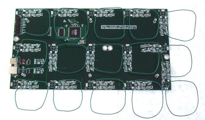
Figure: The A3032 Equipped with Large Wire Coils.
We test the above set of coils in a faraday enclosure with the door closed. We have no additional absorbers. It is immediately apparent that the distribution of coil power is better behaved. The example below is typical for the beaker near the left center of the platform.
Figure: Coil Powers with Large Wire Coils. Note the new "Auto Calib" button, which turns on and off the automatic calibration of power measurements using background power stored with the ALT clock messages.
It takes us ten minutes of moving the beaker before we discover an orientation of the beaker over coil No8 that gives nearly equal power over coil No2, which is 16 cm away. But we are never able to get the power in a coil more than 16 cm away to equal that of the nearby coil. Compared to the original detector coils, the spurious measurements appear to be ten times less frequent. We introduce absorbers, but these do not eliminate the spurious power measurements.
[31-MAR-17] We have submitted the following Antenna Array (A303202A) printed circuit board for fabrication. The board is 40 cm × 23.6 cm. It provides fifteen detector antennas each roughly 7 cm in diameter. The circuit will mount on the A3032 by means of the six platform standoffs. The A3032 itself will be the A3032B, identical to the A3032A, but with all fifteen detector coils removed. The fifteen antennas connect to the vacant coil-mounting pads on the A3032B by means of wires running down through holes in the antenna array circuit board. Each hole is 3.2 mm in diameter and acts as the solder pad for either the signal or ground end of an antenna. The antenna array provides a footprint for us to install a damping resistor in the ground connection of each coil. Coils with damping resonate less, which means they are less sensitive in their direction of maximum sensitivity, but more sensitive in their direction of least sensitivity. We ask ION to return their two prototype ALTs so we can equip them with antenna arrays.
[21-APR-17] We have our antenna array circuit boards and we assemble one onto A3032A base V0385 to make an A3032B. We load 51-Ω damping resistors in every coil.
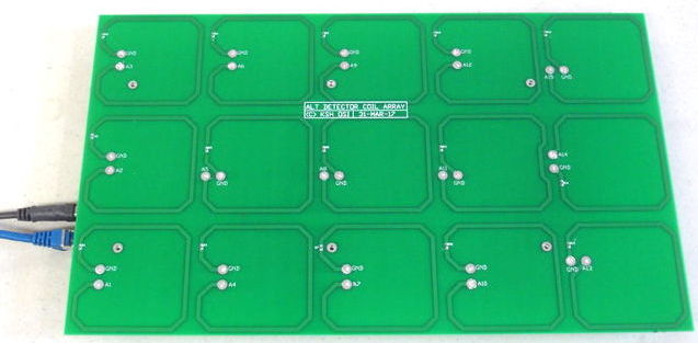
Figure: Animal Location Tracker (A3032B) Platform. The platform is 40 cm × 24 cm.
In a faraday enclosure, we place a dual-channel mouse transmitter on a stand 5 cm high and move it about the platform. For each measurement we place the transmitter above the center of one of the coils in a new orientation. We close the faraday enclosure. We try one hundred locations. The largest position error is 16 cm. The standard deviation of error is around 4 cm. We note that the distribution of powers across the coils is often irregular rather than decreasing with distance from a maximum. With the faraday enclosure door open, we get spurious position measurements far more often, and in one case an error of 32 cm, biased towards the back of the enclosure, away from the door.
[02-MAY-17] We repeat the above experiment with our A3032B, with 51-Ω as before, and also with 0-Ω and ∞-Ω for the damping resistance. Distribution of power in the coils is often irregular. We see maximum error of 16 cm with the faraday enclosure door shut, and 32 cm with the door opening and closing.
We have back from ION A3032As V0383 and V0384. We place V0383 in our faraday enclosure. We turn on a two-channel A3028D rat transmitter and place it in a 50-ml beaker of water supported 30 mm above the platform. We move and rotate the beaker to 100 different positions on the platform.
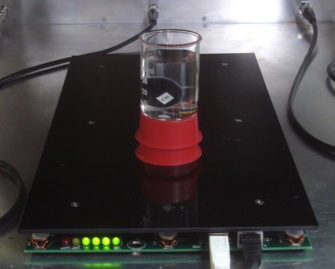
Figure: Test of Distribution and Position.
In each position we close the door and determine whether the distribution of power across the coils is "regular" or "irregular" and whether he position is "correct" or "incorrect". A "regular" distribution is one in which power decreases with range in any particular direction. A "correct" position is any one within an 8-cm radius of the actual position. We perform these observations by visual inspection of the coil power map and the platform. We notice immediately that irregular distributions of power are less frequent with the A3032A/V0383 than with A3032B/V0385. It could be that V0383's amplifiers are more uniform in their gain, or it could be that the small coils are more range-sensitive than the large coils. We embark upon a more thorough study, recording distribution and position for each location.
Figure: Performance Table for 103 Positions, A3032A platform V0383, A3032D transmitter, decreasing power with range criterion for regularity.
The probability of a regular distribution producing a incorrect position is roughly 3%. The probability of an irregular distribution producing an incorrect position is roughly 50%. Ignoring distribution, the probability of a position being incorrect is 16%.
[05-MAY-17] We try our A3032B again. We place our A3028D in water 30 mm above the platform, centered on coil No1. We move the A3028D around for a while with the enclosure door open until we see a spurious position measurement. The measurement depends upon the position of my arm. We record coil power distribution for my left hand on my lap and my left hand 30 cm above my lap. In neither case do we have any part of our body inside the enclosure. In both cases, the coil power distribution is irregular, so we should not trust either position measurement.
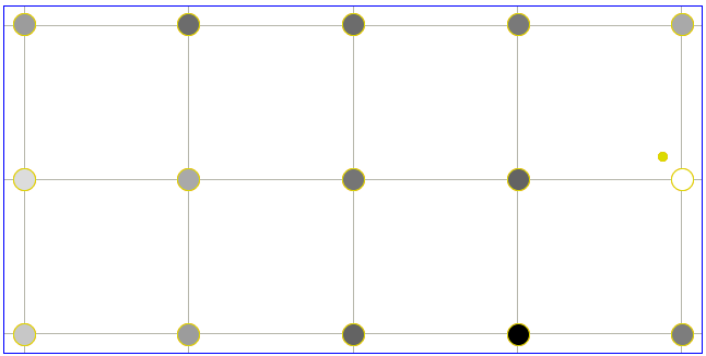
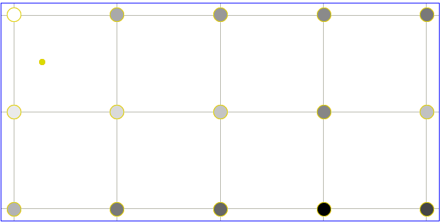
Figure: Coil Powers Before and After 30-cm Move of One Arm Just Outside Enclosure Opening.
The measured position of the A3028D starts off being wrong by 32 cm, and ends being wrong by 16 cm (the platform is 24 cm by 40 cm). We restore the A3028A to the enclosure and attempt to produce the same sensitivity to the position of my arm, but we cannot. We move a 16 cm × 8 cm piece of microwave absorber around in the enclosure, closing the door for each measurement, to see how it affects position, and get the impression that we can disturb the measurement by up to 10 cm in this way, but not 20 cm.
We place a rectangle of absorber on the back wall of our enclosure, so we have the back wall and ceiling absorbing microwaves. We classify the coil power distribution as "regular" if and only if the two coils with the greatest power are immediate neighbors in x or y. A diagonal neighbor does not satisfy this criterion. Position is "correct" if it is within 8 cm.
Figure: Performance Table for 103 Positions, A3032A platform V0383, A3032D transmitter, absorber on back wall, neighboring maxima regularity criterion.
The single regular distribution with incorrect measurement occurred on the front end, opposite the rear wall absorber. Irregular power measurements occurred more frequently when we placed the transmitter above the center of a square made by four coils than when we placed the transmitter directly above a coil.
[09-MAY-17] We move an A3028D in a 50-ml beaker of water 20 mm above the A3032B large-coil platform. We use our near-maximum rule for irregular distribution and 8 cm as the error limit for position to obtain the following performance table. We have no absorber on the back wall.
Figure: Performance Table for 100 Positions, A3032B platform, A3032D transmitter, no absorber on back wall, neighboring maxima criterion.
That's regular with incorrect 14% of the time. We repeat with the transmitter 40 mm above the platform and observe regular with incorrect position 13% of the time in 38 positions. We repeat with 40 mm and an absorber on the back wall an observe 15% irregular and correct in 41 positions. We return to our A3032A platform, V0383 and move the A3028D around in a beaker 20 mm above the surface, with no absorber on the back wall, and our near-maximum criterion. Of 59 positions, we observe 2% (one of them) was regular and incorrect. The following table summarizes our observations.
Figure: Probability that Regular Distribution will produce Position Measurement Within 8 cm of Correct. First row is original regularity criterion, remainder are near-maximum rule.
We conclude that the small coils perform better than the large, and that 20-40 mm altitude and the presence or absence of the absorber have little effect upon the reliability of the measurement.
[26-MAY-17] We enhance lwdaq_locator to accept a percentile parameter. When set to 50, the routine uses the median power in each coil in its weighted centroid calculation. When set to p%, the routine uses the power value for which p% of the samples are less than the power value. We record coil powers while we move a single dual-channel mouse transmitter around in a faraday enclosure. Our recording is M1495564573. At time 47 s the measured position has been stable for twenty seconds and the coil power distribution is regular. We turn off coil calibration and use this processor to obtain, for each coil, a plot of uncalibrated coil power versus percentile value.
Figure: Percentile Power versus Power for All Coils 1-s Interval. Archive M1495564573 time 47 s, regular power distribution and stable location measurement, raw coil powers before calibration.
At 154 s in the same archive, the power distribution is irregular and the location is unstable, jumping 16 cm from one second to the next. We repeat the above experiment and obtain the following plot.
Figure: Percentile Power versus Power for All Coils 1-s Interval. Archive M1495564573 time 154 s, irregular power distribution and unstable location measurement, raw coil powers before calibration.
The increase in power with percentile turns out to be the result of changes in the received power with time during this particular second. We were either opening and closing the door or handling the transmitter. When we plot the median coil power versus time for 154-155 s we get the following progression.
Figure: Median Power versus Time for All Coils. Archive M1495564573 time 154-155 s, irregular power distribution and unstable location measurement, raw coil powers before calibration. Calculate median power for each 1/16 s.
We open a recording of fourteen transmitters on the platform, of which half a dozen are clustered over coil No11 and one, a No12, is over coil 3. We plot coil power versus percentile for 112-113 s in archive M1475253453.
Figure: Percentile Power versus Power for All Coils 1-s Interval. For transmitter No12. Total of fourteen transmitters on the platform. Archive M1475253453 time 112 s. Raw coil powers, no calibration available in this archive.
The measured power remains constant to ±2 counts from 20-80%. Above 90% we see transmissions from other devices colliding with the transmissions of No12, so that the measured power is greater. Coil No11, for example, has several transmitters nearby, but is far from transmitter No12. From 90-100% its measured power increases from 40-140. Below 5% we start to see a drop caused by bad messages on the No12 channel.
[02-JUN-17] Our analysis now divides each interval into a number of slices. For the the maps below, we used eight slices per one-second interval. The final position is the average of the position obtained from the eight slices. We take the standard deviation of the slice positions to obtain a resolution for the measurement. The resolution is a few millimeters for a stationary transmitter when the faraday enclosure door is closed. When the transmitter is moving with the self-propelled ball, the resolution has a minimum value of 0.2 cm, maximum 14 cm and average 7 cm.
We attach transmitter A3028D No9/10 to a self-propelled 8-cm diameter ball. We put the tracker in a box within our faraday enclosure, so that the walls of the box stop the ball leaving the tracker surface. The transmitter moves in a volume 0 cm ⋚ x ≤ 32 cm and 0 cm ≤ y ≤ 16 cm and height 0-8 cm, but we note that when the transmitter is above the outer 2 cm of the platform, it will always be at least 2 cm above the platform. The plot below shows the measured movement of the transmitter during the 600-s recording M1496436129.
Figure: Tracker Movement with Self-Propelled Ball Over Entire Platform. Positions measured every second. The dual-channel transmitter provides two separate position traces. Fort the same recording analyzed without auto-calibration see here.
The ball propels itself randomly with a rotating weight. Sometimes it will shift back and forth for a few seconds, other times it will proceed diagonally 40 cm across the entire platform in less than one second. We introduce a barrier that restricts the ball to the x > 16 cm half of the platform and repeat our experiment with 600-s recording M1496436865.
Figure: Tracker Movement with Self-Propelled Ball Over Half Platform. Positions measured every second from dual-channel transmitter. For the same recording analyzed without auto-calibration see here.
When we compare the movement maps with and without auto-calibration, we note that there are fewer spurious positions without auto-calibration, but the range of the movement is biased away from places we know the ball visits occasionally.
[06-JUN-17] We have archive M1496439825, 300 s from A3028A No11/12 in a 50-mm beaker of water supported 30 mm above the platform. We open our faraday enclosure and move the transmitter from one position to another. From 250-300 s the actual location is (4 cm, 12 cm) and we open and close the enclosure door. We see the following variation in background power obtained during 1-s intervals.
Figure: Variation in Coil Background Power With Opening and Closing of Door. The signal trace is the coil power we receive when the transmitter is emitting power. Traces named after the time in seconds during our recording.
The variations persist regardless of whether we use the minimum, median, or maximum background power measurement. With auto-calibration enabled, in which we subtract these background powers from our transmitter power measurements, we see during this 50-s period the measured location changing by 20 cm. With auto-calibration disabled, the variation is only a few millimeters. Using the minimum background power and 16-s intervals the variation is less than ±1 mm.
We have firmware P3032A08 in which we encode the average background power values we obtain when we place the tracker in a sealed faraday enclosure with no transmitters. Variation in position as we open and close the enclosure door is usually a few millimeters. Near the corners, we see up to 40 mm change with door movement. The 40 mm persists whether we use the minimum, median, or maximum coil power. Thus the apparent change in position is due to an actual change in the power received by the coils from the transmitter, not an addition to the power by interference.
We return to our recording M1496436865 and re-analyze with auto-calibration, 1/16 s intervals, and only one slice per interval. The transmitter is always on the right side of the platform, but is measured as being on the left side 3% of the time.
Figure: Tracker Movement with Self-Propelled Ball Over Half Platform. Positions measured every 1/16 second from channel No9 only.
We consider whether or not the distribution of coil powers can give us a clue as to whether or not a measurement is reliable or not. We plot a graph of coil power versus range from measured position in the Neuroarchiver's value versus time display using a processor you will find in here. We fit a straight line to the graph and consider the slope of the line as an indication of quality of measurement. The more negative the slope, the better the measurement. We go through 200 s of M1496436865, transmitter moving on the right side of the platform, in 1/16-s intervals. We have 83 measurements, or 2.6%, that are on the left side of the platform, which are certainly incorrect. The average slope of the straight line is −0.9 counts/cm for the 83 inaccurate measurements and −1.7 for the remainder. If we ask that the slope be less than −1.1 count/cm, we reject 46% of these 83 measurements, but also 19% of all the remaining measurements. At a threshold of −1.5 we reject 65% and 44% respectively. We try slope divided by residual but obtain no better performance.
[07-JUN-17] Instead of calculating position by weighted centroid, we find the location that maximizes the downward slope of the line we fit to the coil power versus range from location. For 130 s of M1496436865, transmitter moving on the right side of the platform, we obtain this map. When we minimize the slope divided by residual for 100 s, we get this map. We compare intervals in which the two calculations, weighted centroid and slope maximization, lie outside the right half. In roughly 50% of these intervals, both the calculations arrive at the same incorrect answer to within 3 cm of one another, and within the left half. Thus we are unable to use a comparison of the two to eliminate bad measurements. The median separation between the two calculated positions is 4 cm when the weighted centroid is in the right half of the platform.
[08-JUN-17] We implement a new display of location history, in which we make a small, hollow rectangular mark at each location, but plot no path. The following plots shows the position calculated for every 1/16-s interval in the full 600 s of our right-side-only self-propelled ball recording for three different values of the decade scale. The larger the decade scale, the less weight is given to differences in coil power.
Figure: Tracker Movement with Self-Propelled Ball Over Half Platform. Recording M1496436865. Decade scale 20 counts (top), 32 counts (middle), and 50 counts (bottom). Positions measured every 1/16 second from channel No9 only and plotted each as a small square. Centroid extent is 12 cm.
The measured location stays away from the centers of the squares made by the tracker coil grid. Artifacts of the coil arrangement in the distribution of locations become more pronounced as we increase the decade scale. We vary the centroid_extent using a decade scale of 20 and obtain the following plots.
Figure: Tracker Movement with Self-Propelled Ball Over Half Platform. Recording M1496436865. Centroid extent 12 cm (top), 20 cm (middle), and 100 cm (bottom). Positions measured every 1/16 second from channel No9 only and plotted each as a small square. Decade scale is 20 counts.
We analyze our recording of the transmitter moving over the entire platform with centroid extent 12 cm and decade scale 50 counts. We obtain the following map in which coil-induced patterns are clear.
Figure: Tracker Movement with Self-Propelled Ball Over Entire Platform. Recording M1496436129. Decade scale 50 counts, centroid extent 12 cm.
[20-JUN-17] We have a recording M1496930348 made with the A3032B, V0385. We re-program and calibrate its coils in an empty faraday enclosure. During the recording we hold one A3028A No11/12 in a beaker of water 1-4 cm above the platform. For 0-20 s we move the beaker +-1 cm over center of coil 1. For 20-40 s over coil 4. We proceed in order 1, 4, 7, 10, 13, 14, 11, 8, 5, 2, 3, 6, 9, 12, 15. Ending at 300 s.
Figure: Circling By Hand Above Consecutive Coils. From A3032B, centroid extent 12 cm, decade scale 20 counts. Top 201-299 s spending 20 s over each coil in the top row. Center: 101-199 s spending 20 s over each coil along the middle row. Bottom: 0-99 s spending 20 s over each coil along the bottom row.
We try the same experiment with the A3032A, V0383. We make recording M1497988575. The first 100 s is shown below, where we alternate the color of the map for each location.
Figure: Circling By Hand Above Consecutive Coils. From A3032A, centroid extent 12 cm, decade scale 20 counts. 0-99 s spending 20 s over each coil along the bottom row.
[21-JUN-17] Continuing with M1497988575 in 1/16-s intervals, when we vary the centroid extent and the decade scale, our errors increase. We try again our measurement of coil power distribution: the slope of coil power versus range from measured position. We expect this slope to be negative, so if it is positive, we imagine we can assume the location measurement is unreliable. We look at the first twenty seconds of our recording, when we are rotating the transmitter above coil No1. We do not know the exact position of the transmitter, but it lies within 2 cm of coil No1. For the purpose of our plot, we assume the position is exactly over coil No1 and so assume the location error is the distance from No1 to the measured location.
Figure: Location Error versus Slope of Coil Power with Apparent Range. We fit coil power to distance from the measured position.
The slope shows no correlation with measurement error. We look at the standard deviation of the residuals to the straight line fit and obtain this plot showing no correlation. We look at the maximum coil power minus the minimum coil power and obtain this plot showing no correlation. But the plot of error versus maximum coil power shows a slight correlation.
Figure: Location Error versus Maximum Coil Power.
In all nineteen intervals in which the maximum power is ≥95, the maximum power occurs in coil No1, over which we are moving the transmitter. We plot error versus the separation of the two coils with the highest power, as in our "neighboring maxima" criterion, and obtain no correlation. We divide each 1/16th interval into four slices so as to obtain an estimate of the measurement resolution. We see no correlation between location error and estimated resolution from the slices.
[27-JUN-17] We place A3028A No13/14 in a 50-ml beaker of water 40 mm above the A3030A platform at x=16 cm, y=8cm. We record position and plot. Every twenty seconds we move a 200-ml beaker of water to a new position on the platform around the transmitter.
Figure: Effect of Moving a 200-ml Beaker of Water around Transmitter at Platform Center.
Power received by the coil under the transmitter is 110 counts above threshold. The standard deviation of position is around 1 cm. We move the transmitter to x=4cm y=4cm.
Figure: Effect of Moving a 200-ml Beaker of Water around Transmitter at Platform Center.
The power received by the coils around the transmitter reaches a maximum of 90 counts above threshold. The power in the bottom-left corner is as low as 18 and never rises higher than 50. The standard deviation of position is around 10 cm.
We implement a coil power threshold to eliminate measurements with inadequate coil power. We try a threshold on the maximum coil power. But such a threshold favors measurements that are directly over one of the coils. We try a threshold on the total power recorded by the coils, by adding their measurements together, but this does not work because the measurements are logarithmic.
[18-AUG-17] We place a camera above our V0383, A3032A tracking platform. On the platform we place a 15-mm layer of foam and a sheet of 1-cm square graph paper. The camera is equipped with a fish-eye lense. We place two A3028A two-channel mouse transmitters in two petri dishes with glowing LEDs as identifiers for the camera.
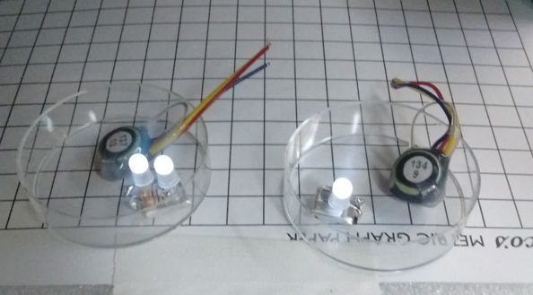
Figure: Marked Transmitters. Transmitter A137.13 is accompanied by two glowing LEDs, and A154.9 by one LED.
Our camera obtains images like this, in which we apply a spot-finding routine to locate the three brightest spots in the image, calculate their positions, and mark them with red squares.
Figure: Photograph of Tracker Platform From Above. We have found the three LEDs automatically. The pair of LEDs tell the location of A137.13. The single LED tells us the location of A154.9.
With the help of a Toolmaker script, we measure the location of each LED in the image. We use the Neurotracker to measure the location of the two transmitters. We write the positions of the three LEDs and the transmitters to a file. We move the transmitters around, sometimes at the same time, sometimes individually, sometimes together, sometimes separately, and we leave them stationary together and separately, taking measurements as we go, until we accumulate 130 measurements of position with the camera and A3032A.
With another script we use the fact that the two closest LEDs are in the same dish to obtain the position of the single and double LED dishes. We also obtain the tracker-measured position of A137.9 and A154.13. We write this condensed data to a file.
Figure: Path of Transmitters According to Camera. We give the position of the LED images on the image sensor in microns, where x and y are parallel to and in the same direction as the ALT x and y.
With another script we select a sub-interval of our 130 movement history and we calculate the correlation between the movement of of each dish and the movement of each transmitter according to the ALT. We have the correlation between the single-LED dish and A137.9, between the single-LED dish and A154.13, between the double-LED dish and A137.9, and between the double-LED dish and A154.13. Although we know already which device is which in the camera image, let us imagine that we do not know, and we want to use these correlations to resolve ambiguity in the camera image as to which transmitter is in which petri dish.
We apply some simple rules to decide if the correlation values are likely to yield an accurate determination. If either dish has no correlation with a transmitter that is above a threshold, we deem the interval to be ambiguous. If a dish has a positive correlation with both transmitters, one must be 20% greater than the other or else they are ambiguous. Assuming the interval is not ambiguous, we have a correct determination only if the correlations of both dishes identify the correct transmitter. Otherwise we have an error.
We select one thousand intervals from our 130-point movement history, each with minimum length ten points. Of the one thousand, 823 are unambiguous and 177 are ambiguous. Of 823 ambiguous intervals, 100.0% give the correct determination of transmitter and dish. With a minimum interval length of 8 or higher, we get 100.0% accuracy. With minimum length 4, we get 3 errors out of 818 intervals, and 182 ambiguous intervals. It appears we will be able to resolve ambiguity in blob-tracking by a camera looking down from the top of the cage with a fish-eye camera.
If we were to place a camera looking from the long side of the platform, it would measure the bearing of the animals with respect to its lens, which would be neither x nor y exactly, but a combination of the two. Suppose we had our camera sufficiently far from the long edge of the platform that the camera x was a good measure of platform x. Can we still resolve ambiguity using only the x-coordinate? We calculate correlation using only the x coordinate of the camera and ALT and get 235 ambiguous, 761 correct, 4 errors with a minimum interval length of 10 points. Thus it appears likely we can resolve ambiguity in video taken from the side of an animal cage.
[23-AUG-17] We attempt to re-calibrate all three of our ALTs, but we find the calibration is unstable. It turns out that we are calibrating the reception of interference within our faraday enclosure. A better way to calibrate would be to excite each coil with the same power source and see how the power measurement varies from coil to coil.
We support an A3028E 20 mm above V0383, an A3032A. We center the transmitter body over coil No1 with the antenna loop in a horizontal plane. As we rotate the transmitter over the coil, the received power varies from 100-140 counts. We place the transmitter over each of the fifteen coils, oriented with respect to each coil so as to give the maximum received power. The maximum for each coil ranges from 130-140 counts. For each coil, the orientation that gives maximum power is the same with respect to the orientation of the coil on the circuit board. We do the same for V0384 and the maxima are 131-144 except for coil No13, for which the maximum is 90. We find an un-soldered pin in the No13 amplifier, correct, and now get maximum power 138 from No13.
Our V0385 is an A3032B with the larger platform and antennas. Variation in coil No1 with rotation is 92-122, although the range over which it is less than 102 is only 20°. Maximum power for all coils is 118-142. For each coil, the maximum power orientation varies from coil to coil in a pattern we cannot identify.
We turn off self-calibration and perform the same disambiguation test upon V0385, A3032B as we did for V0383, A3032A a few days ago, with camera looking down from above, but with two A3028E transmitters in place of two A3028As. We take 48 points, and we have the transmitter supported by 5 cm of foam. With minimum interval 8 we get 161 ambiguous intervals, 833 correct, and 6 errors. When we increase the minimum interval to 9, we get 170 ambiguous, 830 correct, and 0 wrong. During the experiment, every half-dozen movements would be reported by the Neurotracker to be opposite to the direction we had moved it.
We place the same 5-cm foam over V0384, A3032A. We find that the tracking of movement is poor with centroid extent 12 cm. We set centroid extent to 100 cm, so all coil powers will take part in the centroid calculation. Now we find that the direction of movement measured by the tracker is far better correlated with the direction seen by the camera. We take 117 points. Several times we leave the transmitters stationary for four points, but no longer than four. We calculate disambiguation performance for intervals of length 2-12.
| Minimum Length | Correct | Incorrect | Ambiguous |
|---|
| 2 | 873 | 2 | 125 |
| 3 | 901 | 1 | 98 |
| 4 | 913 | 2 | 85 |
| 5 | 915 | 3 | 82 |
| 6 | 945 | 0 | 55 |
| 7 | 950 | 0 | 50 |
| 8 | 956 | 0 | 44 |
| 9 | 952 | 0 | 48 |
| 10 | 961 | 2 | 37 |
| 11 | 975 | 0 | 25 |
| 12 | 964 | 1 | 35 |
| 13 | 972 | 1 | 27 |
| 14 | 972 | 0 | 28 |
| 15 | 980 | 0 | 20 |
| 16 | 985 | 0 | 15 |
| 17 | 985 | 0 | 15 |
| 18 | 991 | 0 | 9 |
| 19 | 991 | 0 | 9 |
| 20 | 994 | 0 | 6 |
Table: Performance of A3032A at Height 5 cm as a Function of Minimum Interval Length. Centroid extent is 100 cm, power threshold 30 counts, power calibration disabled, decade scale 20 counts.
We repeat the V0385, A3032B test with centroid extent 100 cm, hoping to see an improvement in performance, but we once again find that one in every half-dozen movements of each dish is reported by the Neurotracker as being opposite to what we see in the camera. We remove the antenna platform of V0385 and re-assemble as A3032C, where all coils are 33 nH instead of the 257 nH of the A3032A. We support a transmitter 20 mm above coil No1 with the antenna loop in a horizontal plane. We measure power as we rotate the transmitter and see variation 95-144 counts. We repeat for all coils and see maximum power 142-155 counts, except for No7 and No10 which give roughly 100 counts. We re-solder the new inductors and clean and dry. Now all coils within range 142-155 counts maximum power.
We measure the disambiguation performance of V0385, now A3032C, with the transmitter 5 cm above the platform. We move the dishes together for several stretches of five points. We leave them stationary while moving our hand around inside for several stretches of five points. We take a total of 138 points and obtain the following result.
| Minimum Length | Correct | Incorrect | Ambiguous |
|---|
| 2 | 899 | 5 | 96 |
| 3 | 878 | 4 | 118 |
| 4 | 881 | 4 | 115 |
| 5 | 902 | 6 | 92 |
| 6 | 907 | 9 | 84 |
| 7 | 899 | 3 | 98 |
| 8 | 906 | 5 | 89 |
| 9 | 915 | 2 | 83 |
| 10 | 933 | 2 | 65 |
| 11 | 930 | 0 | 70 |
| 12 | 928 | 0 | 72 |
| 13 | 923 | 0 | 77 |
| 14 | 946 | 0 | 54 |
| 15 | 945 | 0 | 55 |
| 16 | 952 | 0 | 48 |
| 17 | 948 | 0 | 52 |
| 18 | 966 | 0 | 34 |
| 19 | 959 | 0 | 41 |
| 20 | 958 | 0 | 42 |
Table: Performance of A3032C at Height 5 cm as a Function of Minimum Interval Length. Centroid extent is 100 cm, power threshold 30 counts, power calibration disabled, decade scale 20 counts.
The number of ambiguous intervals is greater, then in our equivalent test with the A3032A, which we expect, because we moved the transmitters around together more often. The error rate is comparable or better than that of the A3032A.
We set the power calibration of all coils to 20 counts in all three of our ALTs, and in our firmware, and set the default value of auto calibrate to zero in the Neurotracker. The power calibration is not necessary, and appears to have been misguided.
2018
[13-APR-18] We ship V0385, which we have been using here for several months, back to ION along with a Cage Camera (A3034X).
2019
[04-OCT-19] We mount a No4 512 SPS transmitter on the back of a toy mouse, we turn it on for intermittent movement, place it on the ALT platform, cover with upside-down plastic tub to keep it on the platform, and recorded with ALT. Every couple of minutes we have to open Faraday enclosure and jog toy so it will start up again. We can tell when the toy's motor is on by the large amplitude that appears on the EEG signal. We record for ten minutes. Afterwards we use this processor to extract location and signal amplitude for 1/16 s intervals.
set power [Neuroarchiver_band_power 10 160 0 0]
set amplitude [expr sqrt($power)*2.6*1e6/65536/100]
append result "$info(channel_num) $info(tracker_x) $info(tracker_y) [format %0.1f $amplitude] "
We calculate the distance moved in each one-second interval with a Toolmaker script and plot as shown below. They toy moves for five ten-second periods, separated by four ten-second periods of immobility. After that we have to prod the toy to get it to perform another sequence of five movements. When the toy motor is going, the toy does not always move: it sometimes get stuck in the corner of the lid for a few seconds.
Figure: Activity per Second (mm) and Amplitude (mV) versus Time (s). The amplitude rises when the transmitter is moving, because the two electrodes are vibrating in air. The activity is the length of the path traced by sixteen tracker positions obtained within each second.
When the transmitter is not moving, its measured activity is a few millimeters per second. We zoom in to see how well the activity correlates with amplitude in the interval 250-350 s and we can see clearly the five periods of movement, and the correlation between amplitude and activity.
Figure: Activity per Second (mm) and Amplitude (mV) versus Time (s). The amplitude rises when the transmitter is moving, because the two electrodes are vibrating in air. The activity is the length of the path traced by sixteen tracker positions obtained within each second.
We tape another transmitter to the underside of the cover so that it is 10 cm above the platform. The moving toy does not touch the stationary transmitter, but passes under it, so that its body lies between the stationary transmitter and the closest detector coils. The stationary transmitter moves only when we have to pick up the cover to prod the moving toy, which we do after every lull of 20 s or more in its movement. Our purpose is to determine in the worst case how much the movement of one animal will affect the activity we measure for a stationary animal.
Figure: Activity per Second (mm) of Stationary Transmitter and Amplitude (mV) versus Time (s). The amplitude rises when another transmitter is moving on the platform, because this movement vibrates the electrodes of the stationary transmitter. We lift the cover and prod the moving toy at times marked P, in which process we also move the stationary transmitter.
When both transmitters are stationary, the measured activity for the one taped to the cover is a few millimeters per second. When the other transmitter is moving at around 100 mm/s, the measured activity for the stationary transmitter rises at times to 10 mm/s. The background activity roughly 3 mm/s. The crosstalk between activity of two animals is in the worst case 10%.
[17-DEC-19] We remove power calibration entirely from the PO3032A09 firmware. We trust to the accuracy of the LT5534 and the consistency of gain of UPC2746 taken from the same reel when damped by precision LAT-3+ attenuators. We set the payload of the clock messages to zero, except the last byte, which is the firmware version of the notifying receiver. The final byte of all other message is zero also. These bytes are reserved for future use. We play around with several transmitters on an A3032C and find that we get smoother location measurement variation with actual position when we use decade scale 32, rather than our previous preferred value of 20. We are using 8 slices to accelerate calculation and provide us with a precision. Now that we are not subtracting background power, our power threshold is at 60. We leave the extent at 100 so that all coils are used.
2020
[14-JUL-20] We apply a −6 dBm sweep 840-980 MHz to a Loop Antenna (A3015C). We generate the sweep with a Modulating Transmitter (A3014MT), and we split the sweep and mix with 910 MHz to produce an IF ±70 MHz, which we run through a 21-MHz low-pass filter before viewing on the scope. We hold the loop antenna above Coil 10 on V0384 and observer the following response on PW, which is U1004-3.
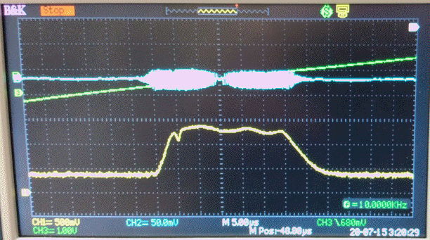
Figure: Sweep Response of Power Measurement. Yellow: PW on U1004-3, 500 mV/div. Green: Ramp voltage that controls A3014MT. Blue: IF reference, center is 910 MHz, left and right edges of bulge are 890 MHz and 930 MHz respectively.
We repeat on all fifteen coils and find the same response on each one, ±100 mV variation in 890-930 MHz, which is roughly ±3 dB. We remove the A3051C loop antenna and replace it with a 3-dB attenuator and a 50-mm bent wire antenna. We observe the same ±3 dB variation on power through the pass band. But in rare orientations of the antenna, all surrounding objects remaining stationary, received power drops suddenly, and variation is ±6 dB.
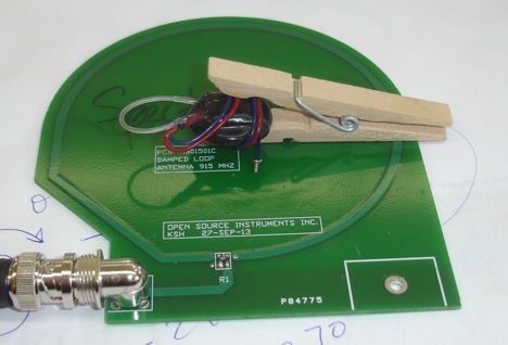
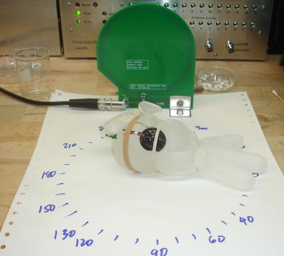